Encyclopedia

Schur complement

Tool in linear algebra and matrix analysis

Wikipedia contributorsAdapted for Fathomly · View authors

4 min read
Source updated October 29, 2025

The Schur complement is a key tool in the fields of linear algebra, the theory of matrices, numerical analysis, and statistics.

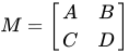
It is defined for a block matrix. Suppose p, q are nonnegative integers such that p + q > 0, and suppose A, B, C, D are respectively p × p, p × q, q × p, and q × q matrices of complex numbers. Let $M={\begin{bmatrix}A&B\\C&D\end{bmatrix}}$ so that M is a (p + q) × (p + q) matrix.

If D is invertible, then the Schur complement of the block D of the matrix M is the p × p matrix defined by $M/D:=A-BD^{-1}C.$ If A is invertible, the Schur complement of the block A of the matrix M is the q × q matrix defined by $M/A:=D-CA^{-1}B.$ In the case that A or D is singular, substituting a generalized inverse for the inverses on M/A and M/D yields the generalized Schur complement.

The Schur complement is named after Issai Schur who used it to prove Schur's lemma, although it had been used previously. Emilie Virginia Haynsworth was the first to call it the Schur complement. The Schur complement is sometimes referred to as the Feshbach map after a physicist Herman Feshbach.

01Background

The Schur complement arises when performing a block Gaussian elimination on the matrix M. In order to eliminate the elements below the block diagonal, one multiplies the matrix M by a block lower triangular matrix on the right as follows: ${\begin{aligned}&M={\begin{bmatrix}A&B\\C&D\end{bmatrix}}\quad \to \quad {\begin{bmatrix}A&B\\C&D\end{bmatrix}}{\begin{bmatrix}I_{p}&0\\-D^{-1}C&I_{q}\end{bmatrix}}={\begin{bmatrix}A-BD^{-1}C&B\\0&D\end{bmatrix}},\end{aligned}}$ where I_p denotes a p×p identity matrix. As a result, the Schur complement $M/D=A-BD^{-1}C$ appears in the upper-left p×p block.

Continuing the elimination process beyond this point (i.e., performing a block Gauss-Jordan elimination), ${\begin{aligned}&{\begin{bmatrix}A-BD^{-1}C&B\\0&D\end{bmatrix}}\quad \to \quad {\begin{bmatrix}I_{p}&-BD^{-1}\\0&I_{q}\end{bmatrix}}{\begin{bmatrix}A-BD^{-1}C&B\\0&D\end{bmatrix}}={\begin{bmatrix}A-BD^{-1}C&0\\0&D\end{bmatrix}},\end{aligned}}$ leads to an LDU decomposition of M, which reads ${\begin{aligned}M&={\begin{bmatrix}A&B\\C&D\end{bmatrix}}={\begin{bmatrix}I_{p}&BD^{-1}\\0&I_{q}\end{bmatrix}}{\begin{bmatrix}A-BD^{-1}C&0\\0&D\end{bmatrix}}{\begin{bmatrix}I_{p}&0\\D^{-1}C&I_{q}\end{bmatrix}}.\end{aligned}}$ Thus, the inverse of M may be expressed involving D⁻¹ and the inverse of Schur's complement, assuming it exists, as ${\begin{aligned}M^{-1}={\begin{bmatrix}A&B\\C&D\end{bmatrix}}^{-1}={}&\left({\begin{bmatrix}I_{p}&BD^{-1}\\0&I_{q}\end{bmatrix}}{\begin{bmatrix}A-BD^{-1}C&0\\0&D\end{bmatrix}}{\begin{bmatrix}I_{p}&0\\D^{-1}C&I_{q}\end{bmatrix}}\right)^{-1}\\={}&{\begin{bmatrix}I_{p}&0\\-D^{-1}C&I_{q}\end{bmatrix}}{\begin{bmatrix}\left(A-BD^{-1}C\right)^{-1}&0\\0&D^{-1}\end{bmatrix}}{\begin{bmatrix}I_{p}&-BD^{-1}\\0&I_{q}\end{bmatrix}}\\[4pt]={}&{\begin{bmatrix}\left(A-BD^{-1}C\right)^{-1}&-\left(A-BD^{-1}C\right)^{-1}BD^{-1}\\-D^{-1}C\left(A-BD^{-1}C\right)^{-1}&D^{-1}+D^{-1}C\left(A-BD^{-1}C\right)^{-1}BD^{-1}\end{bmatrix}}\\[4pt]={}&{\begin{bmatrix}\left(M/D\right)^{-1}&-\left(M/D\right)^{-1}BD^{-1}\\-D^{-1}C\left(M/D\right)^{-1}&D^{-1}+D^{-1}C\left(M/D\right)^{-1}BD^{-1}\end{bmatrix}}.\end{aligned}}$ The above relationship comes from the elimination operations that involve D⁻¹ and M/D. An equivalent derivation can be done with the roles of A and D interchanged. By equating the expressions for M⁻¹ obtained in these two different ways, one can establish the matrix inversion lemma, which relates the two Schur complements of M: M/D and M/A (see "Derivation from LDU decomposition" in Woodbury matrix identity § Alternative proofs).

02Properties

If p and q are both 1 (i.e., A, B, C and D are all scalars), we get the familiar formula for the inverse of a 2-by-2 matrix:

$M^{-1}={\frac {1}{AD-BC}}\left[{\begin{matrix}D&-B\\-C&A\end{matrix}}\right]$

provided that AD − BC is non-zero.

In general, if A is invertible, then

${\begin{aligned}M&={\begin{bmatrix}A&B\\C&D\end{bmatrix}}={\begin{bmatrix}I_{p}&0\\CA^{-1}&I_{q}\end{bmatrix}}{\begin{bmatrix}A&0\\0&D-CA^{-1}B\end{bmatrix}}{\begin{bmatrix}I_{p}&A^{-1}B\\0&I_{q}\end{bmatrix}},\\[4pt]M^{-1}&={\begin{bmatrix}A^{-1}+A^{-1}B(M/A)^{-1}CA^{-1}&-A^{-1}B(M/A)^{-1}\\-(M/A)^{-1}CA^{-1}&(M/A)^{-1}\end{bmatrix}}\end{aligned}}$

whenever this inverse exists.

(Schur's formula) When A, respectively D, is invertible, the determinant of M is also clearly seen to be given by

$\det(M)=\det(A)\det \left(D-CA^{-1}B\right)$ , respectively

$\det(M)=\det(D)\det \left(A-BD^{-1}C\right)$ ,

which generalizes the determinant formula for 2 × 2 matrices.

(Guttman rank additivity formula) If D is invertible, then the rank of M is given by

$\operatorname {rank} (M)=\operatorname {rank} (D)+\operatorname {rank} \left(A-BD^{-1}C\right)$

(Haynsworth inertia additivity formula) If A is invertible, then the inertia of the block matrix M is equal to the inertia of A plus the inertia of M/A.
(Quotient identity) $A/B=((A/C)/(B/C))$ .
The Schur complement of a Laplacian matrix is also a Laplacian matrix.

03Application to solving linear equations

The Schur complement arises naturally in solving a system of linear equations such as

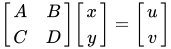
${\begin{bmatrix}A&B\\C&D\end{bmatrix}}{\begin{bmatrix}x\\y\end{bmatrix}}={\begin{bmatrix}u\\v\end{bmatrix}}$ .

Assuming that the submatrix $A$ is invertible, we can eliminate $x$ from the equations, as follows.

$x=A^{-1}(u-By).$

Substituting this expression into the second equation yields

$\left(D-CA^{-1}B\right)y=v-CA^{-1}u.$

We refer to this as the reduced equation obtained by eliminating $x$ from the original equation. The matrix appearing in the reduced equation is called the Schur complement of the first block $A$ in $M$ :

$S\ {\overset {\underset {\mathrm {def} }{}}{=}}\ D-CA^{-1}B$ .

Solving the reduced equation, we obtain

$y=S^{-1}\left(v-CA^{-1}u\right).$

Substituting this into the first equation yields

$x=\left(A^{-1}+A^{-1}BS^{-1}CA^{-1}\right)u-A^{-1}BS^{-1}v.$

We can express the above two equation as:

${\begin{bmatrix}x\\y\end{bmatrix}}={\begin{bmatrix}A^{-1}+A^{-1}BS^{-1}CA^{-1}&-A^{-1}BS^{-1}\\-S^{-1}CA^{-1}&S^{-1}\end{bmatrix}}{\begin{bmatrix}u\\v\end{bmatrix}}.$

Therefore, a formulation for the inverse of a block matrix is:

${\begin{bmatrix}A&B\\C&D\end{bmatrix}}^{-1}={\begin{bmatrix}A^{-1}+A^{-1}BS^{-1}CA^{-1}&-A^{-1}BS^{-1}\\-S^{-1}CA^{-1}&S^{-1}\end{bmatrix}}={\begin{bmatrix}I_{p}&-A^{-1}B\\&I_{q}\end{bmatrix}}{\begin{bmatrix}A^{-1}&\\&S^{-1}\end{bmatrix}}{\begin{bmatrix}I_{p}&\\-CA^{-1}&I_{q}\end{bmatrix}}.$

In particular, we see that the Schur complement is the inverse of the $2,2$ block entry of the inverse of $M$ .

In practice, one needs $A$ to be well-conditioned in order for this algorithm to be numerically accurate.

This method is useful in electrical engineering to reduce the dimension of a network's equations. It is especially useful when element(s) of the output vector are zero. For example, when $u$ or $v$ is zero, we can eliminate the associated rows of the coefficient matrix without any changes to the rest of the output vector. If $v$ is null then the above equation for $x$ reduces to $x=\left(A^{-1}+A^{-1}BS^{-1}CA^{-1}\right)u$ , thus reducing the dimension of the coefficient matrix while leaving $u$ unmodified. This is used to advantage in electrical engineering where it is referred to as node elimination or Kron reduction.

04Applications to probability theory and statistics

Suppose the random column vectors X, Y live in Rⁿ and R^m respectively, and the vector (X, Y) in R^{n + m} has a multivariate normal distribution whose covariance is the symmetric positive-definite matrix

$\Sigma =\left[{\begin{matrix}A&B\\B^{\mathrm {T} }&C\end{matrix}}\right],$

where ${\textstyle A\in \mathbb {R} ^{n\times n}$ is the covariance matrix of X, ${\textstyle C\in \mathbb {R} ^{m\times m}$ is the covariance matrix of Y and ${\textstyle B\in \mathbb {R} ^{n\times m}$ is the covariance matrix between X and Y.

Then the conditional covariance of X given Y is the Schur complement of C in ${\textstyle \Sigma$ :

${\begin{aligned}\operatorname {Cov} (X\mid Y)&=A-BC^{-1}B^{\mathrm {T} }\\\operatorname {E} (X\mid Y)&=\operatorname {E} (X)+BC^{-1}(Y-\operatorname {E} (Y))\end{aligned}}$

If we take the matrix $\Sigma$ above to be, not a covariance of a random vector, but a sample covariance, then it may have a Wishart distribution. In that case, the Schur complement of C in $\Sigma$ also has a Wishart distribution.

05Conditions for positive definiteness and semi-definiteness

Let X be a symmetric matrix of real numbers given by $X=\left[{\begin{matrix}A&B\\B^{\mathrm {T} }&C\end{matrix}}\right].$ Then by the Haynsworth inertia additivity formula, we find

If A is invertible, then X is positive definite if and only if A and its complement X/A are both positive definite:

X\succ 0\Leftrightarrow A\succ 0,X/A=C-B^{\mathrm {T} }A^{-1}B\succ 0.

If C is invertible, then X is positive definite if and only if C and its complement X/C are both positive definite:

X\succ 0\Leftrightarrow C\succ 0,X/C=A-BC^{-1}B^{\mathrm {T} }\succ 0.

If A is positive definite, then X is positive semi-definite if and only if the complement X/A is positive semi-definite:

{\text{If }}A\succ 0,{\text{ then }}X\succeq 0\Leftrightarrow X/A=C-B^{\mathrm {T} }A^{-1}B\succeq 0.

If C is positive definite, then X is positive semi-definite if and only if the complement X/C is positive semi-definite:

{\text{If }}C\succ 0,{\text{ then }}X\succeq 0\Leftrightarrow X/C=A-BC^{-1}B^{\mathrm {T} }\succeq 0.

The first and third statements can also be derived by considering the minimizer of the quantity $u^{\mathrm {T} }Au+2v^{\mathrm {T} }B^{\mathrm {T} }u+v^{\mathrm {T} }Cv,\,$ as a function of v (for fixed u).

Furthermore, since $\left[{\begin{matrix}A&B\\B^{\mathrm {T} }&C\end{matrix}}\right]\succ 0\Longleftrightarrow \left[{\begin{matrix}C&B^{\mathrm {T} }\\B&A\end{matrix}}\right]\succ 0$ and similarly for positive semi-definite matrices, the second (respectively fourth) statement is immediate from the first (resp. third) statement.

There is also a sufficient and necessary condition for the positive semi-definiteness of X in terms of a generalized Schur complement. Precisely,

$X\succeq 0\Leftrightarrow A\succeq 0,C-B^{\mathrm {T} }A^{g}B\succeq 0,\left(I-AA^{g}\right)B=0\,$ and
$X\succeq 0\Leftrightarrow C\succeq 0,A-BC^{g}B^{\mathrm {T} }\succeq 0,\left(I-CC^{g}\right)B^{\mathrm {T} }=0,$

where $A^{g}$ denotes a generalized inverse of $A$ .

Watch videos about Schur complementExplainers and documentaries on YouTube (opens in a new tab)

Sources and credits

This article is adapted from the Wikipedia article “Schur complement”, written by its contributors and licensed under CC BY-SA 4.0. Fathomly has changed the layout, removed citation markers, navigation and maintenance notices, and adjusted punctuation. This adapted version is shared under the same license. For references, see the original article.

Fathomly is not affiliated with or endorsed by the Wikimedia Foundation. Spotted a problem? Tell us.

Schur complement

01Background

02Properties

03Application to solving linear equations

04Applications to probability theory and statistics

05Conditions for positive definiteness and semi-definiteness

Sources and credits

Related topics

Woodbury matrix identity

Quasi-Newton method

Haynsworth inertia additivity formula