Encyclopedia

Multivariate random variable

Random variable with multiple component dimensions

Wikipedia contributorsAdapted for Fathomly · View authors

6 min read
Source updated May 6, 2026

In probability and statistics, a multivariate random variable or random vector is a list or vector of mathematical variables each of whose value is unknown, either because the value has not yet occurred or because there is imperfect knowledge of its value. The individual variables in a random vector are grouped together because they are all part of a single mathematical system, often they represent different properties of an individual statistical unit. For example, while a given person has a specific age, height and weight, the representation of these features of an unspecified person from within a group would be a random vector. Normally each element of a random vector is a real number.

Random vectors are often used as the underlying implementation of various types of aggregate random variables, e.g. a random matrix, random tree, random sequence, stochastic process, etc.

Formally, a multivariate random variable is a column vector $\mathbf {X} =(X_{1},\dots ,X_{n})^{\mathsf {T}}$ (or its transpose, which is a row vector) whose components are random variables on the probability space $(\Omega ,{\mathcal {F}},P)$ , where $\Omega$ is the sample space, ${\mathcal {F}}$ is the sigma-algebra (the collection of all events), and $P$ is the probability measure (a function returning each event's probability).

01Probability distribution

Every random vector gives rise to a probability measure on $\mathbb {R} ^{n}$ with the Borel algebra as the underlying sigma-algebra. This measure is also known as the joint probability distribution, the joint distribution, or the multivariate distribution of the random vector.

The distributions of each of the component random variables $X_{i}$ are called marginal distributions. The conditional probability distribution of $X_{i}$ given $X_{j}$ is the probability distribution of $X_{i}$ when $X_{j}$ is known to be a particular value.

The cumulative distribution function $F_{\mathbf {X} }:\mathbb {R} ^{n}\mapsto [0,1]$ of a random vector $\mathbf {X} =(X_{1},\dots ,X_{n})^{\mathsf {T}}$ is defined as

$F_{\mathbf {X} }(\mathbf {x} )=\operatorname {P} (X_{1}\leq x_{1},\ldots ,X_{n}\leq x_{n})$

Eq.1

where $\mathbf {x} =(x_{1},\dots ,x_{n})^{\mathsf {T}}$ .

02Operations on random vectors

Random vectors can be subjected to the same kinds of algebraic operations as can non-random vectors: addition, subtraction, multiplication by a scalar, and the taking of inner products.

Affine transformations

Similarly, a new random vector $\mathbf {Y}$ can be defined by applying an affine transformation $g\colon \mathbb {R} ^{n}\to \mathbb {R} ^{n}$ to a random vector $\mathbf {X}$ :

$\mathbf {Y} =\mathbf {A} \mathbf {X} +b$ , where $\mathbf {A}$ is an $n\times n$ matrix and $b$ is an $n\times 1$ column vector.

If $\mathbf {A}$ is an invertible matrix and $\textstyle \mathbf {X}$ has a probability density function $f_{\mathbf {X} }$ , then the probability density of $\mathbf {Y}$ is

$f_{\mathbf {Y} }(y)={\frac {f_{\mathbf {X} }(\mathbf {A} ^{-1}(y-b))}{|\det \mathbf {A} |}}$ .

Invertible mappings

More generally we can study invertible mappings of random vectors.

Let $g$ be a one-to-one mapping from an open subset ${\mathcal {D}}$ of $\mathbb {R} ^{n}$ onto a subset ${\mathcal {R}}$ of $\mathbb {R} ^{n}$ , let $g$ have continuous partial derivatives in ${\mathcal {D}}$ and let the Jacobian determinant $\det \left({\frac {\partial \mathbf {y} }{\partial \mathbf {x} }}\right)$ of $g$ be zero at no point of ${\mathcal {D}}$ . Assume that the real random vector $\mathbf {X}$ has a probability density function $f_{\mathbf {X} }(\mathbf {x} )$ and satisfies $P(\mathbf {X} \in {\mathcal {D}})=1$ . Then the random vector $\mathbf {Y} =g(\mathbf {X} )$ is of probability density

$\left.f_{\mathbf {Y} }(\mathbf {y} )={\frac {f_{\mathbf {X} }(\mathbf {x} )}{\left|\det \left({\frac {\partial \mathbf {y} }{\partial \mathbf {x} }}\right)\right|}}\right|_{\mathbf {x} =g^{-1}(\mathbf {y} )}\mathbf {1} (\mathbf {y} \in R_{\mathbf {Y} })$

where $\mathbf {1}$ denotes the indicator function and set $R_{\mathbf {Y} }=\{\mathbf {y} =g(\mathbf {x} ):f_{\mathbf {X} }(\mathbf {x} )>0\}\subseteq {\mathcal {R}}$ denotes support of $\mathbf {Y}$ .

03Expected value

The expected value or mean of a random vector $\mathbf {X}$ is a fixed vector $\operatorname {E} [\mathbf {X} ]$ whose elements are the expected values of the respective random variables.

$\operatorname {E} [\mathbf {X} ]=(\operatorname {E} [X_{1}],...,\operatorname {E} [X_{n}])^{\mathrm {T} }$

Eq.2

04Covariance and cross-covariance

Definitions

The covariance matrix (also called second central moment or variance-covariance matrix) of an $n\times 1$ random vector is an $n\times n$ matrix whose (i,j)^th element is the covariance between the i^th and the j^th random variables. The covariance matrix is the expected value, element by element, of the $n\times n$ matrix computed as $[\mathbf {X} -\operatorname {E} [\mathbf {X} ]][\mathbf {X} -\operatorname {E} [\mathbf {X} ]]^{T}$ , where the superscript T refers to the transpose of the indicated vector:

$\operatorname {K} _{\mathbf {X} \mathbf {X} }=\operatorname {Var} [\mathbf {X} ]=\operatorname {E} [(\mathbf {X} -\operatorname {E} [\mathbf {X} ])(\mathbf {X} -\operatorname {E} [\mathbf {X} ])^{T}]=\operatorname {E} [\mathbf {X} \mathbf {X} ^{T}]-\operatorname {E} [\mathbf {X} ]\operatorname {E} [\mathbf {X} ]^{T}$

Eq.3

By extension, the cross-covariance matrix between two random vectors $\mathbf {X}$ and $\mathbf {Y}$ ( $\mathbf {X}$ having $n$ elements and $\mathbf {Y}$ having $p$ elements) is the $n\times p$ matrix

$\operatorname {K} _{\mathbf {X} \mathbf {Y} }=\operatorname {Cov} [\mathbf {X} ,\mathbf {Y} ]=\operatorname {E} [(\mathbf {X} -\operatorname {E} [\mathbf {X} ])(\mathbf {Y} -\operatorname {E} [\mathbf {Y} ])^{T}]=\operatorname {E} [\mathbf {X} \mathbf {Y} ^{T}]-\operatorname {E} [\mathbf {X} ]\operatorname {E} [\mathbf {Y} ]^{T}$

Eq.4

where again the matrix expectation is taken element-by-element in the matrix. Here the (i,j)^th element is the covariance between the i^th element of $\mathbf {X}$ and the j^th element of $\mathbf {Y}$ .

Properties

The covariance matrix is a symmetric matrix, i.e.

$\operatorname {K} _{\mathbf {X} \mathbf {X} }^{T}=\operatorname {K} _{\mathbf {X} \mathbf {X} }$ .

The covariance matrix is a positive semidefinite matrix, i.e.

$\mathbf {a} ^{T}\operatorname {K} _{\mathbf {X} \mathbf {X} }\mathbf {a} \geq 0\quad {\text{for all }}\mathbf {a} \in \mathbb {R} ^{n}$ .

The cross-covariance matrix $\operatorname {Cov} [\mathbf {Y} ,\mathbf {X} ]$ is simply the transpose of the matrix $\operatorname {Cov} [\mathbf {X} ,\mathbf {Y} ]$ , i.e.

$\operatorname {K} _{\mathbf {Y} \mathbf {X} }=\operatorname {K} _{\mathbf {X} \mathbf {Y} }^{T}$ .

Uncorrelatedness

Two random vectors $\mathbf {X} =(X_{1},...,X_{m})^{T}$ and $\mathbf {Y} =(Y_{1},...,Y_{n})^{T}$ are called uncorrelated if

$\operatorname {E} [\mathbf {X} \mathbf {Y} ^{T}]=\operatorname {E} [\mathbf {X} ]\operatorname {E} [\mathbf {Y} ]^{T}$ .

They are uncorrelated if and only if their cross-covariance matrix $\operatorname {K} _{\mathbf {X} \mathbf {Y} }$ is zero.

05Correlation and cross-correlation

Definitions

The correlation matrix (also called second moment) of an $n\times 1$ random vector is an $n\times n$ matrix whose (i,j)^th element is the correlation between the i^th and the j^th random variables. The correlation matrix is the expected value, element by element, of the $n\times n$ matrix computed as $\mathbf {X} \mathbf {X} ^{T}$ , where the superscript T refers to the transpose of the indicated vector:

$\operatorname {R} _{\mathbf {X} \mathbf {X} }=\operatorname {E} [\mathbf {X} \mathbf {X} ^{\mathrm {T} }]$

Eq.5

By extension, the cross-correlation matrix between two random vectors $\mathbf {X}$ and $\mathbf {Y}$ ( $\mathbf {X}$ having $n$ elements and $\mathbf {Y}$ having $p$ elements) is the $n\times p$ matrix

$\operatorname {R} _{\mathbf {X} \mathbf {Y} }=\operatorname {E} [\mathbf {X} \mathbf {Y} ^{T}]$

Eq.6

Properties

The correlation matrix is related to the covariance matrix by

$\operatorname {R} _{\mathbf {X} \mathbf {X} }=\operatorname {K} _{\mathbf {X} \mathbf {X} }+\operatorname {E} [\mathbf {X} ]\operatorname {E} [\mathbf {X} ]^{T}$ .

Similarly for the cross-correlation matrix and the cross-covariance matrix:

$\operatorname {R} _{\mathbf {X} \mathbf {Y} }=\operatorname {K} _{\mathbf {X} \mathbf {Y} }+\operatorname {E} [\mathbf {X} ]\operatorname {E} [\mathbf {Y} ]^{T}$

06Orthogonality

Two random vectors of the same size $\mathbf {X} =(X_{1},...,X_{n})^{T}$ and $\mathbf {Y} =(Y_{1},...,Y_{n})^{T}$ are called orthogonal if

$\operatorname {E} [\mathbf {X} ^{T}\mathbf {Y} ]=0$ .

07Independence

Two random vectors $\mathbf {X}$ and $\mathbf {Y}$ are called independent if for all $\mathbf {x}$ and $\mathbf {y}$

$F_{\mathbf {X,Y} }(\mathbf {x,y} )=F_{\mathbf {X} }(\mathbf {x} )\cdot F_{\mathbf {Y} }(\mathbf {y} )$

where $F_{\mathbf {X} }(\mathbf {x} )$ and $F_{\mathbf {Y} }(\mathbf {y} )$ denote the cumulative distribution functions of $\mathbf {X}$ and $\mathbf {Y}$ and $F_{\mathbf {X,Y} }(\mathbf {x,y} )$ denotes their joint cumulative distribution function. Independence of $\mathbf {X}$ and $\mathbf {Y}$ is often denoted by $\mathbf {X} \perp \!\!\!\perp \mathbf {Y}$ . Written component-wise, $\mathbf {X}$ and $\mathbf {Y}$ are called independent if for all $x_{1},\ldots ,x_{m},y_{1},\ldots ,y_{n}$

$F_{X_{1},\ldots ,X_{m},Y_{1},\ldots ,Y_{n}}(x_{1},\ldots ,x_{m},y_{1},\ldots ,y_{n})=F_{X_{1},\ldots ,X_{m}}(x_{1},\ldots ,x_{m})\cdot F_{Y_{1},\ldots ,Y_{n}}(y_{1},\ldots ,y_{n})$ .

08Characteristic function

The characteristic function of a random vector $\mathbf {X}$ with $n$ components is a function $\mathbb {R} ^{n}\to \mathbb {C}$ that maps every vector $\mathbf {\omega } =(\omega _{1},\ldots ,\omega _{n})^{T}$ to a complex number. It is defined by

$\varphi _{\mathbf {X} }(\mathbf {\omega } )=\operatorname {E} \left[e^{i(\mathbf {\omega } ^{T}\mathbf {X} )}\right]=\operatorname {E} \left[e^{i(\omega _{1}X_{1}+\ldots +\omega _{n}X_{n})}\right]$ .

09Further properties

Expectation of a quadratic form

One can take the expectation of a quadratic form in the random vector $\mathbf {X}$ as follows:

$\operatorname {E} [\mathbf {X} ^{T}A\mathbf {X} ]=\operatorname {E} [\mathbf {X} ]^{T}A\operatorname {E} [\mathbf {X} ]+\operatorname {tr} (AK_{\mathbf {X} \mathbf {X} }),$

where $K_{\mathbf {X} \mathbf {X} }$ is the covariance matrix of $\mathbf {X}$ and $\operatorname {tr}$ refers to the trace of a matrix, that is, to the sum of the elements on its main diagonal (from upper left to lower right). Since the quadratic form is a scalar, so is its expectation.

Proof: Let $\mathbf {z}$ be an $m\times 1$ random vector with $\operatorname {E} [\mathbf {z} ]=\mu$ and $\operatorname {Cov} [\mathbf {z} ]=V$ and let $A$ be an $m\times m$ non-stochastic matrix.

Then based on the formula for the covariance, if we denote $\mathbf {z} ^{T}=\mathbf {X}$ and $\mathbf {z} ^{T}A^{T}=\mathbf {Y}$ , we see that:

$\operatorname {Cov} [\mathbf {X} ,\mathbf {Y} ]=\operatorname {E} [\mathbf {X} \mathbf {Y} ^{T}]-\operatorname {E} [\mathbf {X} ]\operatorname {E} [\mathbf {Y} ]^{T}$

Hence

${\begin{aligned}\operatorname {E} [XY^{T}]&=\operatorname {Cov} [X,Y]+\operatorname {E} [X]\operatorname {E} [Y]^{T}\\\operatorname {E} [z^{T}Az]&=\operatorname {Cov} [z^{T},z^{T}A^{T}]+\operatorname {E} [z^{T}]\operatorname {E} [z^{T}A^{T}]^{T}\\&=\operatorname {Cov} [z^{T},z^{T}A^{T}]+\mu ^{T}(\mu ^{T}A^{T})^{T}\\&=\operatorname {Cov} [z^{T},z^{T}A^{T}]+\mu ^{T}A\mu ,\end{aligned}}$

which leaves us to show that

$\operatorname {Cov} [z^{T},z^{T}A^{T}]=\operatorname {tr} (AV).$

This is true based on the fact that one can cyclically permute matrices when taking a trace without changing the result (e.g.: $\operatorname {tr} (AB)=\operatorname {tr} (BA)$ ).

We see that

${\begin{aligned}\operatorname {Cov} [z^{T},z^{T}A^{T}]&=\operatorname {E} \left[\left(z^{T}-E(z^{T})\right)\left(z^{T}A^{T}-E\left(z^{T}A^{T}\right)\right)^{T}\right]\\&=\operatorname {E} \left[(z^{T}-\mu ^{T})(z^{T}A^{T}-\mu ^{T}A^{T})^{T}\right]\\&=\operatorname {E} \left[(z-\mu )^{T}(Az-A\mu )\right].\end{aligned}}$

And since

$\left({z-\mu }\right)^{T}\left({Az-A\mu }\right)$

is a scalar, then

$(z-\mu )^{T}(Az-A\mu )=\operatorname {tr} \left({(z-\mu )^{T}(Az-A\mu )}\right)=\operatorname {tr} \left((z-\mu )^{T}A(z-\mu )\right)$

trivially. Using the permutation we get:

$\operatorname {tr} \left({(z-\mu )^{T}A(z-\mu )}\right)=\operatorname {tr} \left({A(z-\mu )(z-\mu )^{T}}\right),$

and by plugging this into the original formula we get:

${\begin{aligned}\operatorname {Cov} \left[{z^{T},z^{T}A^{T}}\right]&=E\left[{\left({z-\mu }\right)^{T}(Az-A\mu )}\right]\\&=E\left[\operatorname {tr} \left(A(z-\mu )(z-\mu )^{T}\right)\right]\\&=\operatorname {tr} \left({A\cdot \operatorname {E} \left((z-\mu )(z-\mu )^{T}\right)}\right)\\&=\operatorname {tr} (AV).\end{aligned}}$

Expectation of the product of two different quadratic forms

One can take the expectation of the product of two different quadratic forms in a zero-mean Gaussian random vector $\mathbf {X}$ as follows:

$\operatorname {E} \left[(\mathbf {X} ^{T}A\mathbf {X} )(\mathbf {X} ^{T}B\mathbf {X} )\right]=2\operatorname {tr} (AK_{\mathbf {X} \mathbf {X} }BK_{\mathbf {X} \mathbf {X} })+\operatorname {tr} (AK_{\mathbf {X} \mathbf {X} })\operatorname {tr} (BK_{\mathbf {X} \mathbf {X} })$

where again $K_{\mathbf {X} \mathbf {X} }$ is the covariance matrix of $\mathbf {X}$ . Again, since both quadratic forms are scalars and hence their product is a scalar, the expectation of their product is also a scalar.

10Applications

Portfolio theory

In portfolio theory in finance, an objective often is to choose a portfolio of risky assets such that the distribution of the random portfolio return has desirable properties. For example, one might want to choose the portfolio return having the lowest variance for a given expected value. Here the random vector is the vector $\mathbf {r}$ of random returns on the individual assets, and the portfolio return p (a random scalar) is the inner product of the vector of random returns with a vector w of portfolio weights, the fractions of the portfolio placed in the respective assets. Since p = w^T $\mathbf {r}$ , the expected value of the portfolio return is w^TE( $\mathbf {r}$ ) and the variance of the portfolio return can be shown to be w^TCw, where C is the covariance matrix of $\mathbf {r}$ .

Regression theory

In linear regression theory, we have data on n observations on a dependent variable y and n observations on each of k independent variables x_j. The observations on the dependent variable are stacked into a column vector y; the observations on each independent variable are also stacked into column vectors, and these latter column vectors are combined into a design matrix X (not denoting a random vector in this context) of observations on the independent variables. Then the following regression equation is postulated as a description of the process that generated the data:

$y=X\beta +e,$

where β is a postulated fixed but unknown vector of k response coefficients, and e is an unknown random vector reflecting random influences on the dependent variable. By some chosen technique such as ordinary least squares, a vector ${\hat {\beta }}$ is chosen as an estimate of β, and the estimate of the vector e, denoted ${\hat {e}}$ , is computed as

${\hat {e}}=y-X{\hat {\beta }}.$

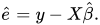
Then the statistician must analyze the properties of ${\hat {\beta }}$ and ${\hat {e}}$ , which are viewed as random vectors since a randomly different selection of n cases to observe would have resulted in different values for them.

Vector time series

The evolution of a k×1 random vector $\mathbf {X}$ through time can be modelled as a vector autoregression (VAR) as follows:

$\mathbf {X} _{t}=c+A_{1}\mathbf {X} _{t-1}+A_{2}\mathbf {X} _{t-2}+\cdots +A_{p}\mathbf {X} _{t-p}+\mathbf {e} _{t},\,$

where the i-periods-back vector observation $\mathbf {X} _{t-i}$ is called the i-th lag of $\mathbf {X}$ , c is a k × 1 vector of constants (intercepts), A_i is a time-invariant k × k matrix and $\mathbf {e} _{t}$ is a k × 1 random vector of error terms.

Watch videos about Multivariate random variableExplainers and documentaries on YouTube (opens in a new tab)

Sources and credits

This article is adapted from the Wikipedia article “Multivariate random variable”, written by its contributors and licensed under CC BY-SA 4.0. Fathomly has changed the layout, removed citation markers, navigation and maintenance notices, and adjusted punctuation. This adapted version is shared under the same license. For references, see the original article.

Images, from Wikimedia Commons:

Standard deviation diagram micro.svg by Ainali, CC BY-SA 3.0

Fathomly is not affiliated with or endorsed by the Wikimedia Foundation. Spotted a problem? Tell us.