Encyclopedia

Covariance

Measure of the joint variability

Wikipedia contributorsAdapted for Fathomly · View authors

9 min read
Source updated May 28, 2026

In probability theory and statistics, covariance is a measure of the joint variability of two random variables. The sign of the covariance shows the tendency in the linear relationship between the variables. Covariance is positive when variables tend to show similar behavior and negative when variables tend to show opposite behavior. The magnitude of the covariance is the geometric mean of the variances that are shared for the two random variables, where a larger magnitude means two variables more strongly depend on each other.

Covariance has units of measurement, and the magnitude of the covariance is affected by said units. This means changing the units (e.g., from meters to millimeters) changes the covariance value proportionally, making it difficult to assess the strength of the relationship from the covariance alone. In some situations, it is desirable to compare the strength of the joint association between different pairs of random variables that do not necessarily have the same units. In those situations, we use the correlation coefficient, which normalizes the covariance to a value between -1 and 1 by dividing by the geometric mean of the total variances (i.e., the product of the standard deviations) for the two random variables.

A distinction is made between (1) the covariance of two random variables, which is a population parameter that can be seen as a property of the joint probability distribution, and (2) the sample covariance, which, in addition to serving as a descriptor of the sample, also serves as an estimated value of the population parameter.

01Definition

For two jointly distributed real-valued random variables $X$ and $Y$ with finite second moments, the covariance is defined as the expected value (or mean) of the product of their deviations from their individual expected values:

$\operatorname {cov} (X,Y)=\operatorname {E} {{\big [}(X-\operatorname {E} [X])(Y-\operatorname {E} [Y]){\big ]}}$

where $\operatorname {E} [X]$ is the expected value of $X$ , also known as the mean of $X$ . The covariance is also sometimes denoted $\sigma _{XY}$ or $\sigma (X,Y)$ , in analogy to variance. By using the linearity property of expectations, this can be simplified to the expected value of their product minus the product of their expected values: ${\begin{aligned}\operatorname {cov} (X,Y)&=\operatorname {E} \left[\left(X-\operatorname {E} \left[X\right]\right)\left(Y-\operatorname {E} \left[Y\right]\right)\right]\\&=\operatorname {E} \left[XY-X\operatorname {E} \left[Y\right]-\operatorname {E} \left[X\right]Y+\operatorname {E} \left[X\right]\operatorname {E} \left[Y\right]\right]\\&=\operatorname {E} \left[XY\right]-\operatorname {E} \left[X\right]\operatorname {E} \left[Y\right]-\operatorname {E} \left[X\right]\operatorname {E} \left[Y\right]+\operatorname {E} \left[X\right]\operatorname {E} \left[Y\right]\\&=\operatorname {E} \left[XY\right]-\operatorname {E} \left[X\right]\operatorname {E} \left[Y\right].\end{aligned}}$ This identity is useful for mathematical derivations. From the viewpoint of numerical computation, however, it is susceptible to catastrophic cancellation (see the section on numerical computation below).

The units of measurement of the covariance $\operatorname {cov} (X,Y)$ are those of $X$ times those of $Y$ . By contrast, correlation coefficients, which depend on the covariance, are a dimensionless measure of linear dependence. (In fact, correlation coefficients can simply be understood as a normalized version of covariance.)

Complex random variables

The covariance between two complex random variables $Z,W$ is defined as $\operatorname {cov} (Z,W)=\operatorname {E} \left[(Z-\operatorname {E} [Z]){\overline {(W-\operatorname {E} [W])}}\right]=\operatorname {E} \left[Z{\overline {W}}\right]-\operatorname {E} [Z]\operatorname {E} \left[{\overline {W}}\right]$

Notice the complex conjugation of the second factor in the definition.

A related pseudo-covariance can also be defined.

Discrete random variables

If the (real) random variable pair $(X,Y)$ can take on the values $(x_{i},y_{i})$ for $i=1,\ldots ,n$ , with equal probabilities $p_{i}=1/n$ , then the covariance can be equivalently written in terms of the means $\operatorname {E} [X]$ and $\operatorname {E} [Y]$ as $\operatorname {cov} (X,Y)={\frac {1}{n}}\sum _{i=1}^{n}(x_{i}-E(X))(y_{i}-E(Y)).$

It can also be equivalently expressed, without directly referring to the means, as $\operatorname {cov} (X,Y)={\frac {1}{n^{2}}}\sum _{i=1}^{n}\sum _{j=1}^{n}{\frac {1}{2}}(x_{i}-x_{j})(y_{i}-y_{j})={\frac {1}{n^{2}}}\sum _{i}\sum _{j>i}(x_{i}-x_{j})(y_{i}-y_{j}).$

More generally, if there are $n$ possible realizations of $(X,Y)$ , namely $(x_{i},y_{i})$ but with possibly unequal probabilities $p_{i}$ for $i=1,\ldots ,n$ , then the covariance is $\operatorname {cov} (X,Y)=\sum _{i=1}^{n}p_{i}(x_{i}-E(X))(y_{i}-E(Y)).$

In the case where two discrete random variables $X$ and $Y$ have a joint probability distribution, represented by elements $p_{i,j}$ corresponding to the joint probabilities of $P(X=x_{i},Y=y_{j})$ , the covariance is calculated using a double summation over the indices of the matrix:

$\operatorname {cov} (X,Y)=\sum _{i=1}^{n}\sum _{j=1}^{n}p_{i,j}(x_{i}-E[X])(y_{j}-E[Y]).$

02Examples

Consider three independent random variables $A,B,C$ and two constants $q,r$ . ${\begin{aligned}X&=qA+B\\Y&=rA+C\\\operatorname {cov} (X,Y)&=qr\operatorname {var} (A)\end{aligned}}$ In the special case, $q=1$ and $r=1$ , the covariance between $X$ and $Y$ is just the variance of $A$ and the name covariance is entirely appropriate.

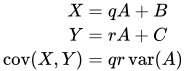
Suppose that $X$ and $Y$ have the following joint probability mass function, in which the six central cells give the discrete joint probabilities $f(x,y)$ of the six hypothetical realizations $(x,y)\in S=\left\{(5,8),(6,8),(7,8),(5,9),(6,9),(7,9)\right\}$ :

$f(x,y)$		5	6	7	$f_{Y}(y)$
$f(x,y)$		x			$f_{Y}(y)$
y	8	0	0.4	0.1	0.5
y	9	0.3	0	0.2	0.5

$f_{X}(x)$		0.3	0.4	0.3	1

$X$ can take on three values (5, 6 and 7) while $Y$ can take on two (8 and 9). Their means are $\mu _{X}=5(0.3)+6(0.4)+7(0.1+0.2)=6$ and $\mu _{Y}=8(0.4+0.1)+9(0.3+0.2)=8.5$ . Then, ${\begin{aligned}\operatorname {cov} (X,Y)={}&\sigma _{XY}=\sum _{(x,y)\in S}f(x,y)\left(x-\mu _{X}\right)\left(y-\mu _{Y}\right)\\[4pt]={}&(0)(5-6)(8-8.5)+(0.4)(6-6)(8-8.5)+(0.1)(7-6)(8-8.5)+{}\\[4pt]&(0.3)(5-6)(9-8.5)+(0)(6-6)(9-8.5)+(0.2)(7-6)(9-8.5)\\[4pt]={}&{-0.1}\;.\end{aligned}}$

03Properties

Covariance with itself

The variance is a special case of the covariance in which the two variables are identical: $\operatorname {cov} (X,X)=\operatorname {var} (X)\equiv \sigma ^{2}(X)\equiv \sigma _{X}^{2}.$

Covariance of linear combinations

If $X$ , $Y$ , $W$ , and $V$ are real-valued random variables and $a,b,c,d$ are real-valued constants, then the following facts are a consequence of the definition of covariance: ${\begin{aligned}\operatorname {cov} (X,a)&=0\\\operatorname {cov} (X,X)&=\operatorname {var} (X)\\\operatorname {cov} (X,Y)&=\operatorname {cov} (Y,X)\\\operatorname {cov} (aX,bY)&=ab\,\operatorname {cov} (X,Y)\\\operatorname {cov} (X+a,Y+b)&=\operatorname {cov} (X,Y)\\\operatorname {cov} (aX+bY,cW+dV)&=ac\,\operatorname {cov} (X,W)+ad\,\operatorname {cov} (X,V)+bc\,\operatorname {cov} (Y,W)+bd\,\operatorname {cov} (Y,V)\end{aligned}}$

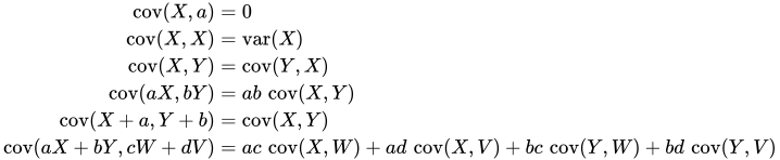
For a sequence $X_{1},\ldots ,X_{n}$ of real-valued random variables and constants $a_{1},\ldots ,a_{n}$ , we have $\operatorname {var} \left(\sum _{i=1}^{n}a_{i}X_{i}\right)=\sum _{i=1}^{n}a_{i}^{2}\operatorname {var} (X_{i})+2\sum _{i,j\,:\,i<j}a_{i}a_{j}\operatorname {cov} (X_{i},X_{j})=\sum _{i,j}{a_{i}a_{j}\operatorname {cov} (X_{i},X_{j})}$

Hoeffding's covariance identity

A useful identity to compute the covariance between two random variables $X,Y$ is the Hoeffding's covariance identity: $\operatorname {cov} (X,Y)=\int _{\mathbb {R} }\int _{\mathbb {R} }\left(F_{(X,Y)}(x,y)-F_{X}(x)F_{Y}(y)\right)\,dx\,dy$ where $F_{(X,Y)}(x,y)$ is the joint cumulative distribution function of the random vector $(X,Y)$ and $F_{X}(x),F_{Y}(y)$ are the marginals.

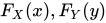
Uncorrelatedness and independence

Random variables whose covariance is zero are called uncorrelated. Similarly, the components of random vectors whose covariance matrix is zero in every entry outside the main diagonal are also called uncorrelated.

If $X$ and $Y$ are independent random variables, then their covariance is zero. This follows because under independence, $\operatorname {E} [XY]=\operatorname {E} [X]\cdot \operatorname {E} [Y].$

The converse, however, is not generally true. For example, let $X$ be uniformly distributed in $[-1,1]$ and let $Y=X^{2}$ . Clearly, $X$ and $Y$ are not independent, but ${\begin{aligned}\operatorname {cov} (X,Y)&=\operatorname {cov} \left(X,X^{2}\right)\\&=\operatorname {E} \left[X\cdot X^{2}\right]-\operatorname {E} [X]\cdot \operatorname {E} \left[X^{2}\right]\\&=\operatorname {E} \left[X^{3}\right]-\operatorname {E} [X]\operatorname {E} \left[X^{2}\right]\\&=0-0\cdot \operatorname {E} [X^{2}]\\&=0.\end{aligned}}$

In this case, the relationship between $Y$ and $X$ is non-linear, while correlation and covariance are measures of linear dependence between two random variables. This example shows that if two random variables are uncorrelated, that does not in general imply that they are independent. However, if two variables are jointly normally distributed (but not if they are merely individually normally distributed), uncorrelatedness does imply independence.

$X$ and $Y$ whose covariance is positive are called positively correlated, which implies if $X>E[X]$ then likely $Y>E[Y]$ . Conversely, $X$ and $Y$ with negative covariance are negatively correlated, and if $X>E[X]$ then likely $Y<E[Y]$ .

Relationship to inner products

Many of the properties of covariance can be extracted elegantly by observing that it satisfies similar properties to those of an inner product:

bilinear: for constants $a$ and $b$ and random variables $X,Y,Z,$ $\operatorname {cov} (aX+bY,Z)=a\operatorname {cov} (X,Z)+b\operatorname {cov} (Y,Z)$
symmetric: $\operatorname {cov} (X,Y)=\operatorname {cov} (Y,X)$
positive semi-definite: $\sigma ^{2}(X)=\operatorname {cov} (X,X)\geq 0$ for all random variables $X$ , and $\operatorname {cov} (X,X)=0$ implies that $X$ is constant almost surely.

In fact these properties imply that the covariance defines an inner product over the quotient vector space obtained by taking the subspace of random variables with finite second moment and identifying any two that differ by a constant. (This identification turns the positive semi-definiteness above into positive definiteness.) That quotient vector space is isomorphic to the subspace of random variables with finite second moment and mean zero; on that subspace, the covariance is exactly the L² inner product of real-valued functions on the sample space.

As a result, for random variables with finite variance, the inequality $\left|\operatorname {cov} (X,Y)\right|\leq {\sqrt {\sigma ^{2}(X)\sigma ^{2}(Y)}}$ is a special case of the Cauchy-Schwarz inequality.

For convenience, here is an explicit proof, which uses only the inner product properties above.

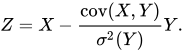
If $\sigma ^{2}(Y)=0$ , then it holds trivially. Otherwise, define the random variable $Z=X-{\frac {\operatorname {cov} (X,Y)}{\sigma ^{2}(Y)}}Y.$

Then we have ${\begin{aligned}0\leq \sigma ^{2}(Z)&=\operatorname {cov} \left(X-{\frac {\operatorname {cov} (X,Y)}{\sigma ^{2}(Y)}}Y,\;X-{\frac {\operatorname {cov} (X,Y)}{\sigma ^{2}(Y)}}Y\right)\\[12pt]&=\sigma ^{2}(X)-{\frac {(\operatorname {cov} (X,Y))^{2}}{\sigma ^{2}(Y)}}\\\implies (\operatorname {cov} (X,Y))^{2}&\leq \sigma ^{2}(X)\sigma ^{2}(Y)\\\left|\operatorname {cov} (X,Y)\right|&\leq {\sqrt {\sigma ^{2}(X)\sigma ^{2}(Y)}}\end{aligned}}$

04Calculating the sample covariance

The sample covariances among $K$ variables based on $N$ observations of each, drawn from an otherwise unobserved population, are given by the $K\times K$ matrix $\textstyle {\overline {\mathbf {q} }}=\left[q_{jk}\right]$ with the entries

$q_{jk}={\frac {1}{N-1}}\sum _{i=1}^{N}\left(X_{ij}-{\bar {X}}_{j}\right)\left(X_{ik}-{\bar {X}}_{k}\right),$

which is an estimate of the covariance between variable $j$ and variable $k$ .

The sample mean and the sample covariance matrix are unbiased estimates of the mean and the covariance matrix of the random vector $\textstyle \mathbf {X}$ , a vector whose jth element $(j=1,\,\ldots ,\,K)$ is one of the random variables. The reason the sample covariance matrix has $\textstyle N-1$ in the denominator rather than $\textstyle N$ is essentially that the population mean $\operatorname {E} (\mathbf {X} )$ is not known and is replaced by the sample mean $\mathbf {\bar {X}}$ . If the population mean $\operatorname {E} (\mathbf {X} )$ is known, the analogous unbiased estimate is given by

$q_{jk}={\frac {1}{N}}\sum _{i=1}^{N}\left(X_{ij}-\operatorname {E} \left(X_{j}\right)\right)\left(X_{ik}-\operatorname {E} \left(X_{k}\right)\right)$ .

05Generalizations

Auto-covariance matrix of real random vectors

For a vector $\mathbf {X} ={\begin{bmatrix}X_{1}&X_{2}&\dots &X_{m}\end{bmatrix}}^{\mathrm {T} }$ of $m$ jointly distributed random variables with finite second moments, its auto-covariance matrix (also known as the variance-covariance matrix or simply the covariance matrix) $\operatorname {K} _{\mathbf {X} \mathbf {X} }$ (also denoted by $\Sigma (\mathbf {X} )$ or $\operatorname {cov} (\mathbf {X} ,\mathbf {X} )$ ) is defined as ${\begin{aligned}\operatorname {K} _{\mathbf {XX} }=\operatorname {cov} (\mathbf {X} ,\mathbf {X} )&=\operatorname {E} \left[(\mathbf {X} -\operatorname {E} [\mathbf {X} ])(\mathbf {X} -\operatorname {E} [\mathbf {X} ])^{\mathrm {T} }\right]\\&=\operatorname {E} \left[\mathbf {XX} ^{\mathrm {T} }\right]-\operatorname {E} [\mathbf {X} ]\operatorname {E} [\mathbf {X} ]^{\mathrm {T} }.\end{aligned}}$

Let $\mathbf {X}$ be a random vector with covariance matrix Σ, and let A be a matrix that can act on $\mathbf {X}$ on the left. The covariance matrix of the matrix-vector product A X is: ${\begin{aligned}\operatorname {cov} (\mathbf {AX} ,\mathbf {AX} )&=\operatorname {E} \left[\mathbf {AX(A} \mathbf {X)} ^{\mathrm {T} }\right]-\operatorname {E} [\mathbf {AX} ]\operatorname {E} \left[(\mathbf {A} \mathbf {X} )^{\mathrm {T} }\right]\\&=\operatorname {E} \left[\mathbf {AXX} ^{\mathrm {T} }\mathbf {A} ^{\mathrm {T} }\right]-\operatorname {E} [\mathbf {AX} ]\operatorname {E} \left[\mathbf {X} ^{\mathrm {T} }\mathbf {A} ^{\mathrm {T} }\right]\\&=\mathbf {A} \operatorname {E} \left[\mathbf {XX} ^{\mathrm {T} }\right]\mathbf {A} ^{\mathrm {T} }-\mathbf {A} \operatorname {E} [\mathbf {X} ]\operatorname {E} \left[\mathbf {X} ^{\mathrm {T} }\right]\mathbf {A} ^{\mathrm {T} }\\&=\mathbf {A} \left(\operatorname {E} \left[\mathbf {XX} ^{\mathrm {T} }\right]-\operatorname {E} [\mathbf {X} ]\operatorname {E} \left[\mathbf {X} ^{\mathrm {T} }\right]\right)\mathbf {A} ^{\mathrm {T} }\\&=\mathbf {A} \Sigma \mathbf {A} ^{\mathrm {T} }.\end{aligned}}$

This is a direct result of the linearity of expectation and is useful when applying a linear transformation, such as a whitening transformation, to a vector.

Cross-covariance matrix of real random vectors

For real random vectors $\mathbf {X} \in \mathbb {R} ^{m}$ and $\mathbf {Y} \in \mathbb {R} ^{n}$ , the $m\times n$ cross-covariance matrix is equal to

${\begin{aligned}\operatorname {K} _{\mathbf {X} \mathbf {Y} }=\operatorname {cov} (\mathbf {X} ,\mathbf {Y} )&=\operatorname {E} \left[(\mathbf {X} -\operatorname {E} [\mathbf {X} ])(\mathbf {Y} -\operatorname {E} [\mathbf {Y} ])^{\mathrm {T} }\right]\\&=\operatorname {E} \left[\mathbf {X} \mathbf {Y} ^{\mathrm {T} }\right]-\operatorname {E} [\mathbf {X} ]\operatorname {E} [\mathbf {Y} ]^{\mathrm {T} }\end{aligned}}$

Eq.2

where $\mathbf {Y} ^{\mathrm {T} }$ is the transpose of the vector (or matrix) $\mathbf {Y}$ .

The $(i,j)$ -th element of this matrix is equal to the covariance $\operatorname {cov} (X_{i},Y_{j})$ between the i-th scalar component of $\mathbf {X}$ and the j-th scalar component of $\mathbf {Y}$ . In particular, $\operatorname {cov} (\mathbf {Y} ,\mathbf {X} )$ is the transpose of $\operatorname {cov} (\mathbf {X} ,\mathbf {Y} )$ .

Cross-covariance sesquilinear form of random vectors in a real or complex Hilbert space

More generally let $H_{1}=(H_{1},\langle \,,\rangle _{1})$ and $H_{2}=(H_{2},\langle \,,\rangle _{2})$ , be Hilbert spaces over $\mathbb {R}$ or $\mathbb {C}$ with $\langle \,,\rangle$ anti linear in the first variable, and let $\mathbf {X} ,\mathbf {Y}$ be $H_{1}$ resp. $H_{2}$ valued random variables. Then the covariance of $\mathbf {X}$ and $\mathbf {Y}$ is the sesquilinear form on $H_{1}\times H_{2}$ (anti linear in the first variable) given by ${\begin{aligned}\operatorname {K} _{X,Y}(h_{1},h_{2})=\operatorname {cov} (\mathbf {X} ,\mathbf {Y} )(h_{1},h_{2})&=\operatorname {E} \left[\langle h_{1},(\mathbf {X} -\operatorname {E} [\mathbf {X} ])\rangle _{1}\langle (\mathbf {Y} -\operatorname {E} [\mathbf {Y} ]),h_{2}\rangle _{2}\right]\\&=\operatorname {E} [\langle h_{1},\mathbf {X} \rangle _{1}\langle \mathbf {Y} ,h_{2}\rangle _{2}]-\operatorname {E} [\langle h,\mathbf {X} \rangle _{1}]\operatorname {E} [\langle \mathbf {Y} ,h_{2}\rangle _{2}]\\&=\langle h_{1},\operatorname {E} \left[(\mathbf {X} -\operatorname {E} [\mathbf {X} ])(\mathbf {Y} -\operatorname {E} [\mathbf {Y} ])^{\dagger }\right]h_{2}\rangle _{1}\\&=\langle h_{1},\left(\operatorname {E} [\mathbf {X} \mathbf {Y} ^{\dagger }]-\operatorname {E} [\mathbf {X} ]\operatorname {E} [\mathbf {Y} ]^{\dagger }\right)h_{2}\rangle _{1}\\\end{aligned}}$

06Numerical computation

When $\operatorname {E} [XY]\approx \operatorname {E} [X]\operatorname {E} [Y]$ , the equation $\operatorname {cov} (X,Y)=\operatorname {E} \left[XY\right]-\operatorname {E} \left[X\right]\operatorname {E} \left[Y\right]$ is prone to catastrophic cancellation if $\operatorname {E} \left[XY\right]$ and $\operatorname {E} \left[X\right]\operatorname {E} \left[Y\right]$ are not computed exactly and thus should be avoided in computer programs when the data has not been centered before. Numerically stable algorithms should be preferred in this case.

07Comments

The covariance is sometimes called a measure of "linear dependence" between the two random variables. That does not mean the same thing as in the context of linear algebra (see linear dependence). When the covariance is normalized, one obtains the Pearson correlation coefficient, which gives the goodness of the fit for the best possible linear function describing the relation between the variables. In this sense covariance is a linear gauge of dependence.

08Applications

Genetics and molecular biology

Covariance is an important measure in biology. Certain sequences of DNA are conserved more than others among species, and thus to study secondary and tertiary structures of proteins, or of RNA structures, sequences are compared in closely related species. If sequence changes are found or no changes at all are found in noncoding RNA (such as microRNA), sequences are found to be necessary for common structural motifs, such as an RNA loop. In genetics, covariance serves a basis for computation of Genetic Relationship Matrix (GRM) (aka kinship matrix), enabling inference on population structure from sample with no known close relatives as well as inference on estimation of heritability of complex traits.

In the theory of evolution and natural selection, the Price equation describes how a genetic trait changes in frequency over time. The equation uses a covariance between a trait and fitness, to give a mathematical description of evolution and natural selection. It provides a way to understand the effects that gene transmission and natural selection have on the proportion of genes within each new generation of a population.

Financial economics

Covariances play a key role in financial economics, especially in modern portfolio theory and in the capital asset pricing model. Covariances among various assets' returns are used to determine, under certain assumptions, the relative amounts of different assets that investors should (in a normative analysis) or are predicted to (in a positive analysis) choose to hold in a context of diversification.

Meteorological and oceanographic data assimilation

The covariance matrix is important in estimating the initial conditions required for running weather forecast models, a procedure known as data assimilation. The "forecast error covariance matrix" is typically constructed between perturbations around a mean state (either a climatological or ensemble mean). The "observation error covariance matrix" is constructed to represent the magnitude of combined observational errors (on the diagonal) and the correlated errors between measurements (off the diagonal). This is an example of its widespread application to Kalman filtering and more general state estimation for time-varying systems.

Micrometeorology

The eddy covariance technique is a key atmospherics measurement technique where the covariance between instantaneous deviation in vertical wind speed from the mean value and instantaneous deviation in gas concentration is the basis for calculating the vertical turbulent fluxes.

Signal processing

The covariance matrix is used to capture the spectral variability of a signal.

09Correlation

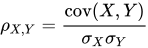
The Pearson product-moment correlation coefficient between two random variables $X$ and $Y$ is defined as $\rho _{X,Y}={\frac {\operatorname {cov} (X,Y)}{\sigma _{X}\sigma _{Y}}}$

where

$\operatorname {cov}$ is the covariance
$\sigma _{X}$ is the standard deviation of $X$
$\sigma _{Y}$ is the standard deviation of $Y$ .

The denominator can also be written as ${\sqrt {\operatorname {var} (X)\operatorname {var} (Y)}}$ , which is the geometric mean of the variances.

Thus we see that the correlation coefficient is a normalized version of the covariance. It is always a number between $-1$ and $1$ , and is unitless (unlike the covariance).

The correlation coefficient is often denoted by r, and is frequently reported in scientific studies.

10Principal component analysis

The covariance matrix is used in principal component analysis to reduce feature dimensionality in data preprocessing. The principal components are the dimensions that explain the most variance in the data. A well known application is to intelligence, producing the g factor. Another is to personality, with models like the five factor model being derived from principal component analysis.

Watch videos about CovarianceExplainers and documentaries on YouTube (opens in a new tab)

Sources and credits

This article is adapted from the Wikipedia article “Covariance”, written by its contributors and licensed under CC BY-SA 4.0. Fathomly has changed the layout, removed citation markers, navigation and maintenance notices, and adjusted punctuation. This adapted version is shared under the same license. For references, see the original article.

Images, from Wikimedia Commons:

Covariance trends.svg by Cmglee, CC BY-SA 4.0
Covariance geometric visualisation.svg by Cmglee, CC BY-SA 4.0

Fathomly is not affiliated with or endorsed by the Wikimedia Foundation. Spotted a problem? Tell us.