Encyclopedia

Estimation theory

Branch of statistics to estimate models based on measured data

Wikipedia contributorsAdapted for Fathomly · View authors

5 min read
Source updated November 27, 2025

Estimation theory is a branch of statistics that deals with estimating the values of parameters based on measured empirical data that has a random component. The parameters describe an underlying physical setting in such a way that their value affects the distribution of the measured data. An estimator attempts to approximate the unknown parameters using the measurements. In estimation theory, two approaches are generally considered:

The probabilistic approach (described in this article) assumes that the measured data is random with a probability distribution dependent on the parameters of interest
The set-membership approach assumes that the measured data vector belongs to a set which depends on the parameter vector.

01Examples

For example, it is desired to estimate the proportion of a population of voters who will vote for a particular candidate. That proportion is the parameter sought; the estimate is based on a small random sample of voters. Alternatively, it is desired to estimate the probability of a voter voting for a particular candidate, based on some demographic features, such as age.

Or, for example, in radar the aim is to find the range of objects (airplanes, boats, etc.) by analyzing the two-way transit timing of received echoes of transmitted pulses. Since the reflected pulses are unavoidably embedded in electrical noise, their measured values are randomly distributed, so that the transit time must be estimated.

As another example, in electrical communication theory, the measurements which contain information regarding the parameters of interest are often associated with a noisy signal.

02Basics

For a given model, several statistical "ingredients" are needed so the estimator can be implemented. The first is a statistical sample, a set of data points taken from a random vector (RV) of size N. Put into a vector, $\mathbf {x} ={\begin{bmatrix}x[0]\\x[1]\\\vdots \\x[N-1]\end{bmatrix}}.$ Secondly, there are M parameters ${\boldsymbol {\theta }}={\begin{bmatrix}\theta _{1}\\\theta _{2}\\\vdots \\\theta _{M}\end{bmatrix}},$ whose values are to be estimated. Third, the continuous probability density function (pdf) or its discrete counterpart, the probability mass function (pmf), of the underlying distribution that generated the data must be stated conditional on the values of the parameters: $p(\mathbf {x} |{\boldsymbol {\theta }}).\,$ It is also possible for the parameters themselves to have a probability distribution (e.g., Bayesian statistics). It is then necessary to define the Bayesian probability $\pi ({\boldsymbol {\theta }}).\,$ After the model is formed, the goal is to estimate the parameters, with the estimates commonly denoted ${\hat {\boldsymbol {\theta }}}$ , where the "hat" indicates the estimate.

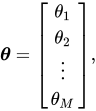
One common estimator is the minimum mean squared error (MMSE) estimator, which utilizes the error between the estimated parameters and the actual value of the parameters $\mathbf {e} ={\hat {\boldsymbol {\theta }}}-{\boldsymbol {\theta }}$ as the basis for optimality. This error term is then squared and the expected value of this squared value is minimized for the MMSE estimator.

03Estimators

Commonly used estimators (estimation methods) and topics related to them include:

Maximum likelihood estimators
Bayes estimators
Method of moments estimators
Cramér-Rao bound
Least squares
Minimum mean squared error (MMSE), also known as Bayes least squared error (BLSE)
Maximum a posteriori (MAP)
Minimum variance unbiased estimator (MVUE)
Nonlinear system identification
Best linear unbiased estimator (BLUE)
Unbiased estimators , see estimator bias.
Particle filter
Markov chain Monte Carlo (MCMC)
Kalman filter, and its various derivatives
Wiener filter

04Examples

Unknown constant in additive white Gaussian noise

Consider a received discrete signal, $x[n]$ , of $N$ independent samples that consists of an unknown constant $A$ with additive white Gaussian noise (AWGN) $w[n]$ with zero mean and known variance $\sigma ^{2}$ (i.e., ${\mathcal {N}}(0,\sigma ^{2})$ ). Since the variance is known then the only unknown parameter is $A$ .

The model for the signal is then $x[n]=A+w[n]\quad n=0,1,\dots ,N-1$

Two possible (of many) estimators for the parameter $A$ are:

${\hat {A}}_{1}=x[0]$
${\hat {A}}_{2}={\frac {1}{N}}\sum _{n=0}^{N-1}x[n]$ which is the sample mean

Both of these estimators have a mean of $A$ , which can be shown through taking the expected value of each estimator $\mathrm {E} \left[{\hat {A}}_{1}\right]=\mathrm {E} \left[x[0]\right]=A$ and $\mathrm {E} \left[{\hat {A}}_{2}\right]=\mathrm {E} \left[{\frac {1}{N}}\sum _{n=0}^{N-1}x[n]\right]={\frac {1}{N}}\left[\sum _{n=0}^{N-1}\mathrm {E} \left[x[n]\right]\right]={\frac {1}{N}}\left[NA\right]=A$

At this point, these two estimators would appear to perform the same. However, the difference between them becomes apparent when comparing the variances. $\mathrm {var} \left({\hat {A}}_{1}\right)=\mathrm {var} \left(x[0]\right)=\sigma ^{2}$ and $\mathrm {var} \left({\hat {A}}_{2}\right)=\mathrm {var} \left({\frac {1}{N}}\sum _{n=0}^{N-1}x[n]\right){\overset {\text{independence}}{=}}{\frac {1}{N^{2}}}\left[\sum _{n=0}^{N-1}\mathrm {var} (x[n])\right]={\frac {1}{N^{2}}}\left[N\sigma ^{2}\right]={\frac {\sigma ^{2}}{N}}$

It would seem that the sample mean is a better estimator since its variance is lower for every N > 1.

Maximum likelihood

Continuing the example using the maximum likelihood estimator, the probability density function (pdf) of the noise for one sample $w[n]$ is $p(w[n])={\frac {1}{\sigma {\sqrt {2\pi }}}}\exp \left(-{\frac {1}{2\sigma ^{2}}}w[n]^{2}\right)$ and the probability of $x[n]$ becomes ( $x[n]$ can be thought of a ${\mathcal {N}}(A,\sigma ^{2})$ ) $p(x[n];A)={\frac {1}{\sigma {\sqrt {2\pi }}}}\exp \left(-{\frac {1}{2\sigma ^{2}}}(x[n]-A)^{2}\right)$ By independence, the probability of $\mathbf {x}$ becomes $p(\mathbf {x} ;A)=\prod _{n=0}^{N-1}p(x[n];A)={\frac {1}{\left(\sigma {\sqrt {2\pi }}\right)^{N}}}\exp \left(-{\frac {1}{2\sigma ^{2}}}\sum _{n=0}^{N-1}(x[n]-A)^{2}\right)$ Taking the natural logarithm of the pdf $\ln p(\mathbf {x} ;A)=-N\ln \left(\sigma {\sqrt {2\pi }}\right)-{\frac {1}{2\sigma ^{2}}}\sum _{n=0}^{N-1}(x[n]-A)^{2}$ and the maximum likelihood estimator is ${\hat {A}}=\arg \max \ln p(\mathbf {x} ;A)$

Taking the first derivative of the log-likelihood function ${\frac {\partial }{\partial A}}\ln p(\mathbf {x} ;A)={\frac {1}{\sigma ^{2}}}\left[\sum _{n=0}^{N-1}(x[n]-A)\right]={\frac {1}{\sigma ^{2}}}\left[\sum _{n=0}^{N-1}x[n]-NA\right]$ and setting it to zero $0={\frac {1}{\sigma ^{2}}}\left[\sum _{n=0}^{N-1}x[n]-NA\right]=\sum _{n=0}^{N-1}x[n]-NA$

This results in the maximum likelihood estimator ${\hat {A}}={\frac {1}{N}}\sum _{n=0}^{N-1}x[n]$ which is simply the sample mean. From this example, it was found that the sample mean is the maximum likelihood estimator for $N$ samples of a fixed, unknown parameter corrupted by AWGN.

Cramér-Rao lower bound

To find the Cramér-Rao lower bound (CRLB) of the sample mean estimator, it is first necessary to find the Fisher information number ${\mathcal {I}}(A)=\mathrm {E} \left(\left[{\frac {\partial }{\partial A}}\ln p(\mathbf {x} ;A)\right]^{2}\right)=-\mathrm {E} \left[{\frac {\partial ^{2}}{\partial A^{2}}}\ln p(\mathbf {x} ;A)\right]$ and copying from above ${\frac {\partial }{\partial A}}\ln p(\mathbf {x} ;A)={\frac {1}{\sigma ^{2}}}\left[\sum _{n=0}^{N-1}x[n]-NA\right]$

Taking the second derivative ${\frac {\partial ^{2}}{\partial A^{2}}}\ln p(\mathbf {x} ;A)={\frac {1}{\sigma ^{2}}}(-N)={\frac {-N}{\sigma ^{2}}}$ and finding the negative expected value is trivial since it is now a deterministic constant $-\mathrm {E} \left[{\frac {\partial ^{2}}{\partial A^{2}}}\ln p(\mathbf {x} ;A)\right]={\frac {N}{\sigma ^{2}}}$

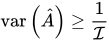
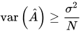
Finally, putting the Fisher information into $\mathrm {var} \left({\hat {A}}\right)\geq {\frac {1}{\mathcal {I}}}$ results in $\mathrm {var} \left({\hat {A}}\right)\geq {\frac {\sigma ^{2}}{N}}$

Comparing this to the variance of the sample mean (determined previously) shows that the sample mean is equal to the Cramér-Rao lower bound for all values of $N$ and $A$ . In other words, the sample mean is the (necessarily unique) efficient estimator, and thus also the minimum variance unbiased estimator (MVUE), in addition to being the maximum likelihood estimator.

Maximum of a uniform distribution

One of the simplest non-trivial examples of estimation is the estimation of the maximum of a uniform distribution. It is used as a hands-on classroom exercise and to illustrate basic principles of estimation theory. Further, in the case of estimation based on a single sample, it demonstrates philosophical issues and possible misunderstandings in the use of maximum likelihood estimators and likelihood functions.

Given a discrete uniform distribution $1,2,\dots ,N$ with unknown maximum, the UMVU estimator for the maximum is given by ${\frac {k+1}{k}}m-1=m+{\frac {m}{k}}-1$ where m is the sample maximum and k is the sample size, sampling without replacement. This problem is commonly known as the German tank problem, due to application of maximum estimation to estimates of German tank production during World War II.

The formula may be understood intuitively as;

"The sample maximum plus the average gap between observations in the sample",

the gap being added to compensate for the negative bias of the sample maximum as an estimator for the population maximum.

This has a variance of ${\frac {1}{k}}{\frac {(N-k)(N+1)}{(k+2)}}\approx {\frac {N^{2}}{k^{2}}}{\text{ for small samples }}k\ll N$ so a standard deviation of approximately $N/k$ , the (population) average size of a gap between samples; compare ${\frac {m}{k}}$ above. This can be seen as a very simple case of maximum spacing estimation.

The sample maximum is the maximum likelihood estimator for the population maximum, but, as discussed above, it is biased.

05Applications

Numerous fields require the use of estimation theory. Some of these fields include:

Interpretation of scientific experiments
Signal processing
Clinical trials
Opinion polls
Quality control
Telecommunications
Project management
Software engineering
Control theory (in particular Adaptive control)
Network intrusion detection system
Orbit determination

Measured data are likely to be subject to noise or uncertainty and it is through statistical probability that optimal solutions are sought to extract as much information from the data as possible.

Watch videos about Estimation theoryExplainers and documentaries on YouTube (opens in a new tab)

Sources and credits

This article is adapted from the Wikipedia article “Estimation theory”, written by its contributors and licensed under CC BY-SA 4.0. Fathomly has changed the layout, removed citation markers, navigation and maintenance notices, and adjusted punctuation. This adapted version is shared under the same license. For references, see the original article.

Fathomly is not affiliated with or endorsed by the Wikimedia Foundation. Spotted a problem? Tell us.