Reference articles on history, science, culture and more
Encyclopedia

Continuous function

Mathematical function with no sudden changes

In mathematics, a continuous function is a function such that a small variation of its argument induces at most a small variation of its value. This implies there are no abrupt changes in value, known as discontinuities. More precisely, a function is continuous if arbitrarily small changes in its value can be assured by restricting its argument to sufficiently small changes. A discontinuous function is a function that is not continuous. Until the 19th century, mathematicians largely relied on intuitive notions of continuity and considered only continuous functions. The epsilon-delta definition of a limit was introduced to formalize the definition of continuity.

Continuity is one of the core concepts of calculus and mathematical analysis, where arguments and values of functions are real numbers and complex numbers. The concept has been generalized to functions between metric spaces and between topological spaces. The latter are the most general continuous functions, and their definition is the basis of topology.

A stronger form of continuity is uniform continuity. In order theory, especially in domain theory, a related concept of continuity is Scott continuity.

As a practical example, the function H(t) denoting the height of a growing flower at time t would be considered continuous. In contrast, the function M(t) denoting the amount of money in a bank account at time t would be considered discontinuous since it "jumps" at each point in time when money is deposited or withdrawn.

01History

A form of the epsilon-delta definition of continuity was first given by Bernard Bolzano in 1817. Augustin-Louis Cauchy defined continuity of y=f(x) as follows: an infinitely small increment \alpha of the independent variable x always produces an infinitely small change f(x+\alpha )-f(x) of the dependent variable y (see e.g. Cours d'Analyse, p. 34). Cauchy defined infinitely small quantities in terms of variable quantities, and his definition of continuity closely parallels the infinitesimal definition used today (see microcontinuity).

The formal definitions for, and distinction between, pointwise continuity and uniform continuity were first given by Bolzano in the 1830s, but the work was not published until the 1930s. Like Bolzano, Karl Weierstrass considered that a function y=f(x) at a point x=c, that is f(x){\big |}_{x=c} , is continuous if and only if the values of f(c), f(x){\big |}_{x\to c^{+}}, and f(x){\big |}_{x\to c^{-}} are all defined and equal. Édouard Goursat assumed continuity provided that the function is defined at f(c) and is equal to at least one side of the limit f(x){\big |}_{x\to c} , whereas Camille Jordan allowed it even if the function was defined only at x=c. All three of these nonequivalent definitions of pointwise continuity are still in use. Eduard Heine provided the first published definition of uniform continuity in 1872, but based these ideas on lectures given by Peter Gustav Lejeune Dirichlet in 1854.

The function is continuous on its domain (), but is discontinuous at when considered as a partial function defined on the reals.
The sequence exp(1/n) converges to exp(0) = 1.

02Real functions

Definition

A real function (that is, a function from real numbers to real numbers) can be represented by a graph in the Cartesian plane; such a function is continuous if, roughly speaking, the graph is a single unbroken curve whose domain is the entire real line. A more mathematically rigorous definition is given below.

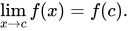
Continuity of real functions is usually defined in terms of limits. A function f with variable x is continuous at the real number c if the limit of f(x), as x tends to c, is equal to f(c).

There are several different definitions of the (global) continuity of a function, which depend on the nature of its domain.

A function is continuous on an open interval if (1) the interval is contained in the function's domain, and (2) the function is continuous at every point in the interval. A function that is continuous on the interval (-\infty ,+\infty ) (the whole real line) is often simply called a continuous function; one also says that such a function is continuous everywhere. For example, all polynomial functions are continuous everywhere.

A function is continuous on a semi-open or a closed interval if (1) the interval is contained in the function's domain, (2) the function is continuous at every point in the interval, and (3) the function is continuous at the closed endpoints, that is, technically, the value of the function at a closed endpoint equals the limit of the values of the function as the variable approaches the endpoint from the interior of the interval. For example, the function f(x)={\sqrt {x}} is continuous on its whole domain, which is the semi-open interval [0,+\infty ).

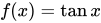
Many commonly encountered functions are partial functions that have a domain formed by all real numbers, except for some isolated points. Examples include the reciprocal function {\textstyle f(x)={\frac {1}{x}} and the tangent function f(x)=\tan x. When these partial functions are continuous on their domain, they are (in some contexts) said to be continuous, although they are not continuous everywhere. In other contexts, mainly when one is interested in their behavior near the exceptional points, they are said to be discontinuous.

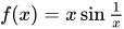
A partial function is discontinuous at a point if the point belongs to the topological closure of its domain, and either the point does not belong to the domain of the function or the function is not continuous at the point. For example, the functions {\textstyle f(x)={\frac {1}{x}} and {\textstyle f(x)=\sin({\frac {1}{x}}) are discontinuous at 0, and remain discontinuous whichever value is chosen for defining them at 0. A point where a function is discontinuous is called a discontinuity. At a point where a function is not defined, and therefore discontinuous, the discontinuity is removable if a value of the function can be chosen at that point to make the function continuous. For example, the function f(x)=x\sin {\tfrac {1}{x}} has a removable discontinuity at zero, since \textstyle \lim _{x\to 0}x\sin {\frac {1}{x}}=0, and the discontinuity at 0 of f(x)=\sin {\tfrac {1}{x}} is not removable, since \textstyle \lim _{x\to 0}\sin {\frac {1}{x}} does not exist.

Using mathematical notation, several ways exist to define continuous functions in the three senses mentioned above.

Let {\textstyle f:D\to \mathbb {R} be a function whose domain D is a subset of the real numbers \mathbb {R} .

Some (but not all) possibilities for D are:

In the case of an open interval, a and b do not belong to D, and the values f(a) and f(b) are not defined, and if they are, they do not matter for continuity on D.

Definition in terms of limits of functions

The function f is continuous at some point c of its domain if the limit of f(x), as x approaches c through the domain of f, exists and is equal to f(c). In mathematical notation, this is written as \lim _{x\to c}{f(x)}=f(c). In detail this means three conditions: first, f has to be defined at c (guaranteed by the requirement that c be in the domain of f). Second, the limit of that equation must exist. Third, the value of this limit must equal f(c).

(Here, we have assumed that the domain of f does not have any isolated points.)

Definition in terms of neighborhoods

A neighborhood of a point c is a set that contains, at least, all points within some fixed distance of c. Intuitively, a function is continuous at a point c if the range of f over the neighborhood of c shrinks to a single point f(c) as the width of the neighborhood around c shrinks to zero. More precisely, a function f is continuous at a point c of its domain if, for any neighborhood N_{1}(f(c)) there is a neighborhood N_{2}(c) in its domain such that f(x)\in N_{1}(f(c)) whenever x\in N_{2}(c).

As neighborhoods are defined in any topological space, this definition of a continuous function applies not only for real functions but also when the domain and the codomain are topological spaces and is thus the most general definition. It follows that a function is automatically continuous at every isolated point of its domain. For example, every real-valued function on the integers is continuous.

Definition in terms of limits of sequences

One can instead require that for any sequence (x_{n})_{n\in \mathbb {N} } of points in the domain which converges to c, the corresponding sequence \left(f(x_{n})\right)_{n\in \mathbb {N} } converges to f(c). In mathematical notation, \forall (x_{n})_{n\in \mathbb {N} }\subset D:\lim _{n\to \infty }x_{n}=c\Rightarrow \lim _{n\to \infty }f(x_{n})=f(c)\,.

Weierstrass and Jordan definitions (epsilon-delta) of continuous functions

Explicitly including the definition of the limit of a function, we obtain a self-contained definition: Given a function f:D\to \mathbb {R} as above and an element x_{0} of the domain D, f is said to be continuous at the point x_{0} when the following holds: For any positive real number \varepsilon >0, however small, there exists some positive real number \delta >0 such that for all x in the domain of f with x_{0}-\delta <x<x_{0}+\delta , the value of f(x) satisfies f\left(x_{0}\right)-\varepsilon <f(x)<f(x_{0})+\varepsilon .

Alternatively written, continuity of f:D\to \mathbb {R} at x_{0}\in D means that for every \varepsilon >0, there exists a \delta >0 such that for all x\in D: \left|x-x_{0}\right|<\delta ~~{\text{ implies }}~~|f(x)-f(x_{0})|<\varepsilon .

More intuitively, we can say that if we want to get all the f(x) values to stay in some small neighborhood around f\left(x_{0}\right), we need to choose a small enough neighborhood for the x values around x_{0}. If we can do that no matter how small the f(x_{0}) neighborhood is, then f is continuous at x_{0}.

In modern terms, this is generalized by the definition of continuity of a function with respect to a basis for the topology, here the metric topology.

Weierstrass had required that the interval x_{0}-\delta <x<x_{0}+\delta be entirely within the domain D, but Jordan removed that restriction.

Definition in terms of control of the remainder

In proofs and numerical analysis, we often need to know how fast limits are converging, or in other words, control of the remainder. We can formalize this to a definition of continuity. A function C:[0,\infty )\to [0,\infty ] is called a control function if C is non-decreasing and \inf _{\delta >0}C(\delta )=0.

A function f:D\to R is C-continuous at x_{0} if there exists a neighborhood {\textstyle N(x_{0}) such that |f(x)-f(x_{0})|\leq C\left(\left|x-x_{0}\right|\right){\text{ for all }}x\in D\cap N(x_{0}).

A function is continuous in x_{0} if it is C-continuous for some control function C.

This approach leads naturally to refining the notion of continuity by restricting the set of admissible control functions. For a given set of control functions {\mathcal {C}}, a function is {\mathcal {C}}-continuous if it is C-continuous for some C\in {\mathcal {C}}. For example, the Lipschitz, the Hölder continuous functions of exponent α and the uniformly continuous functions below are defined by the set of control functions {\mathcal {C}}_{\mathrm {Lipschitz} }=\{C:C(\delta )=K|\delta |,\ K>0\} {\mathcal {C}}_{{\text{Hölder}}-\alpha }=\{C:C(\delta )=K|\delta |^{\alpha },\ K>0\} {\mathcal {C}}_{\text{uniform cont.}}=\{C:C(0)=0\} respectively.

Definition using oscillation

Continuity can also be defined in terms of oscillation: a function f is continuous at a point x_{0} if and only if its oscillation at that point is zero; in symbols, \omega _{f}(x_{0})=0. A benefit of this definition is that it quantifies discontinuity: the oscillation gives how much the function is discontinuous at a point.

This definition is helpful in descriptive set theory to study the set of discontinuities and continuous points, the continuous points are the intersection of the sets where the oscillation is less than \varepsilon (hence a G_{\delta } set), and gives a rapid proof of one direction of the Lebesgue integrability condition.

The oscillation is equivalent to the \varepsilon -\delta definition by a simple re-arrangement and by using a limit (lim sup, lim inf) to define oscillation: if (at a given point) for a given \varepsilon _{0} there is no \delta that satisfies the \varepsilon -\delta definition, then the oscillation is at least \varepsilon _{0}, and conversely if for every \varepsilon there is a desired \delta , the oscillation is 0. The oscillation definition can be naturally generalized to maps from a topological space to a metric space.

Definition using the hyperreals

Cauchy defined the continuity of a function in the following intuitive terms: an infinitesimal change in the independent variable corresponds to an infinitesimal change of the dependent variable (see Cours d'analyse, page 34). Non-standard analysis is a way of making this mathematically rigorous. The real line is augmented by adding infinite and infinitesimal numbers to form the hyperreal numbers. In nonstandard analysis, continuity can be defined as follows.

A real-valued function f is continuous at x if its natural extension to the hyperreals has the property that for all infinitesimal dx, f(x+dx)-f(x) is infinitesimal

(see microcontinuity). In other words, an infinitesimal increment of the independent variable always produces an infinitesimal change of the dependent variable, giving a modern expression to Augustin-Louis Cauchy's definition of continuity.

Rules for continuity

Proving the continuity of a function by a direct application of the definition is generally not an easy task. Fortunately, in practice, most functions are built from simpler functions, and their continuity can be deduced immediately from the way they are defined, by applying the following rules:

  • Every constant function is continuous
  • The identity function f(x)=x is continuous
  • Addition and multiplication: if the functions f and g are continuous on their respective domains D_{f} and D_{g}, then their sum f+g and their product f\cdot g are continuous on the intersection D_{f}\cap D_{g}, where f+g and f\cdot g are defined by (f+g)(x)=f(x)+g(x) and (f\cdot g)(x)=f(x)\cdot g(x).
  • Reciprocal: If the function f is continuous on the domain D_{f}, then its reciprocal {\tfrac {1}{f}}, defined by ({\tfrac {1}{f}})(x)={\tfrac {1}{f(x)}} is continuous on the domain D_{f}\setminus f^{-1}(0), that is, the domain D_{f} from which the points x such that f(x)=0 are removed.
  • Function composition: If the functions f and g are continuous on their respective domains D_{f} and D_{g}, then the composition g\circ f defined by {1} is continuous on D_{f}\cap f^{-1}(D_{g}), that is, the part of D_{f} that is mapped by f inside D_{g}.
  • The sine and cosine functions (\sin x and \cos x) are continuous everywhere.
  • The exponential function e^{x} is continuous everywhere.
  • The natural logarithm \ln x is continuous on the domain formed by all positive real numbers \{x\mid x>0\}.

These rules imply that every polynomial function is continuous everywhere and that a rational function is continuous everywhere where it is defined, if the numerator and the denominator have no common zeros. More generally, the quotient of two continuous functions is continuous outside the zeros of the denominator.

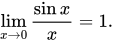
An example of a function for which the above rules are not sufficient is the sinc function, which is defined by \operatorname {sinc} (0)=1 and \operatorname {sinc} (x)={\tfrac {\sin x}{x}} for x\neq 0. The above rules show immediately that the function is continuous for all x\neq 0, but to prove continuity at x=0, one has to prove \lim _{x\to 0}{\frac {\sin x}{x}}=1. This is indeed true, and thus the sinc function is continuous function on all real numbers.

Examples of discontinuous functions

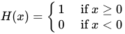
An example of a discontinuous function is the Heaviside step function H, defined by H(x)={\begin{cases}1&{\text{ if }}x\geq 0\\0&{\text{ if }}x<0\end{cases}}

Pick for instance \varepsilon =1/2. Then there is no \delta-neighborhood around x=0, i.e. no open interval (-\delta ,\;\delta ) with \delta >0, that will force all the H(x) values to be within the \varepsilon-neighborhood of H(0), i.e. within (1/2,\;3/2). Intuitively, we can think of this type of discontinuity as a sudden jump in function values.

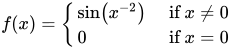
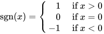
Similarly, the signum or sign function \operatorname {sgn} (x)={\begin{cases}\;\;\ 1&{\text{ if }}x>0\\\;\;\ 0&{\text{ if }}x=0\\-1&{\text{ if }}x<0\end{cases}} is discontinuous at x=0 but continuous everywhere else. Yet another example: the function f(x)={\begin{cases}\sin \left(x^{-2}\right)&{\text{ if }}x\neq 0\\0&{\text{ if }}x=0\end{cases}} is continuous everywhere except x=0.
Besides plausible continuities and discontinuities like above, there are also functions with pathological behavior; for example, Thomae's function, f(x)={\begin{cases}1&{\text{ if }}x=0\\{\frac {1}{q}}&{\text{ if }}x={\frac {p}{q}}{\text{(in lowest terms) is a rational number}}\\0&{\text{ if }}x{\text{ is irrational}}.\end{cases}} is continuous at all irrational numbers and discontinuous at all rational numbers. In a similar vein, Dirichlet's function, the indicator function for the set of rational numbers, D(x)={\begin{cases}0&{\text{ if }}x{\text{  is irrational }}(\in \mathbb {R} \setminus \mathbb {Q} )\\1&{\text{ if }}x{\text{ is rational }}(\in \mathbb {Q} )\end{cases}} is nowhere continuous.

Properties

A useful lemma

Let f(x) be a function that is continuous at a point x_{0}, and y_{0} be a value such f\left(x_{0}\right)\neq y_{0}. Then f(x)\neq y_{0} throughout some neighborhood of x_{0}.

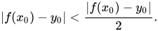
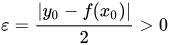
Proof: By the definition of continuity, take \varepsilon ={\frac {|y_{0}-f(x_{0})|}{2}}>0 , then there exists \delta >0 such that \left|f(x)-f(x_{0})\right|<{\frac {\left|y_{0}-f(x_{0})\right|}{2}}\quad {\text{ whenever }}\quad |x-x_{0}|<\delta Suppose there is a point in the neighborhood |x-x_{0}|<\delta for which f(x)=y_{0}; then we have the contradiction \left|f(x_{0})-y_{0}\right|<{\frac {\left|f(x_{0})-y_{0}\right|}{2}}.
Intermediate value theorem

The intermediate value theorem is an existence theorem, based on the real number property of completeness, and states:

If the real-valued function f is continuous on the closed interval [a,b], and k is some number between f(a) and f(b), then there is some number c\in [a,b], such that f(c)=k.

For example, if a child grows from 1 m to 1.5 m between the ages of two and six years, then, at some time between two and six years of age, the child's height must have been 1.25 m.

As a consequence, if f is continuous on [a,b] and f(a) and f(b) differ in sign, then, at some point c\in [a,b], f(c) must equal zero.

Extreme value theorem

The extreme value theorem states that if a function f is defined and continuous on a closed interval [a,b] (or any closed and bounded set), then the function attains its maximum, i.e. there exists c\in [a,b] with f(c)\geq f(x) for all x\in [a,b]. The same is true of the minimum of f. These statements are not, in general, true if the function is defined on an open interval (a,b) (or any set that is not both closed and bounded), as, for example, the continuous function f(x)={\frac {1}{x}}, defined on the open interval (0,1), does not attain a maximum, being unbounded above.

Relation to differentiability and integrability

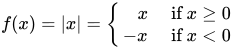
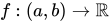
Every differentiable function f:(a,b)\to \mathbb {R} is continuous, as can be shown. The converse does not hold: for example, the absolute value function
f(x)=|x|={\begin{cases}\;\;\ x&{\text{ if }}x\geq 0\\-x&{\text{ if }}x<0\end{cases}}

is everywhere continuous. However, it is not differentiable at x=0 (but is so everywhere else). Weierstrass's function is also everywhere continuous but nowhere differentiable.

The derivative f'(x) of a differentiable function f(x) need not be continuous. If f'(x) is continuous, f(x) is said to be continuously differentiable. The set of such functions is denoted C^{1}((a,b)). More generally, the set of functions f:\Omega \to \mathbb {R} (from an open interval (or open subset of \mathbb {R}) \Omega to the reals) such that f is n times differentiable and such that the n-th derivative of f is continuous is denoted C^{n}(\Omega ); see differentiability class. In the field of computer graphics, properties related (but not identical) to C^{0},C^{1},C^{2} are sometimes called G^{0} (continuity of position), G^{1} (continuity of tangency), and G^{2} (continuity of curvature); see smoothness of curves and surfaces.

Every continuous function f:[a,b]\to \mathbb {R} is integrable (for example in the sense of the Riemann integral). The converse does not hold, as the (integrable but discontinuous) sign function shows.

Pointwise and uniform limits

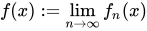
Given a sequence f_{1},f_{2},\dotsc :I\to \mathbb {R} of functions such that the limit f(x):=\lim _{n\to \infty }f_{n}(x) exists for all x\in D, the resulting function f(x) is referred to as the pointwise limit of the sequence of functions \left(f_{n}\right)_{n\in N}. The pointwise limit function need not be continuous, even if all functions f_{n} are continuous, as the animation at the right shows. However, f is continuous if all functions f_{n} are continuous and the sequence converges uniformly, by the uniform convergence theorem. This theorem can be used to show that the exponential functions, logarithms, square root function, and trigonometric functions are continuous.

Directional continuity

Discontinuous functions may be discontinuous in a restricted way, giving rise to the concept of directional continuity (or right- and left-continuous functions) and semi-continuity. Roughly speaking, a function is right-continuous if no jump occurs when the limit point is approached from the right. Formally, f is said to be right-continuous at the point c if the following holds: For any number \varepsilon >0 however small, there exists some number \delta >0 such that for all x in the domain with c<x<c+\delta , the value of f(x) satisfies |f(x)-f(c)|<\varepsilon

This is the same condition as continuous functions, except it is required to hold only for x strictly larger than c. Requiring |f(x)-f(c)|<\varepsilon to hold instead for all x with c-\delta <x<c yields the notion of left-continuous functions. A function is continuous if and only if it is both right-continuous and left-continuous.

Semicontinuity

A function f is lower semi-continuous at the point c if, roughly, any jumps that might occur only go down, but not up. That is, for any \varepsilon >0, there exists some number \delta >0 such that for all x in the domain with |x-c|<\delta , the value of f(x) satisfies f(x)\geq f(c)-\varepsilon . The reverse condition is upper semi-continuity.

Illustration of the ε-δ-definition: at x = 2, any value δ ≤ 0.5 satisfies the condition of the definition for ε = 0.5.
The failure of a function to be continuous at a point is quantified by its oscillation.

03Continuous functions between metric spaces

The concept of continuous real-valued functions can be generalized to functions between metric spaces. A metric space is a set X equipped with a function (called a metric) d_{X}, that can be thought of as a measurement of the distance of any two elements in X. Formally, the metric is a function d_{X}:X\times X\to \mathbb {R} that satisfies a number of requirements, notably the triangle inequality. Given two metric spaces \left(X,d_{X}\right) and \left(Y,d_{Y}\right) and a function f:X\to Y then f is continuous at the point c\in X (with respect to the given metrics) if for any positive real number \varepsilon >0, there exists a positive real number \delta >0 such that all x\in X satisfying d_{X}(x,c)<\delta will also satisfy d_{Y}(f(x),f(c))<\varepsilon . As in the case of real functions above, this is equivalent to the condition that for every sequence \left(x_{n}\right) in X with \lim x_{n}=c, we have \lim f\left(x_{n}\right)=f(c). The latter condition can be weakened as follows: f is continuous at the point c if and only if for every convergent sequence \left(x_{n}\right) in X with limit c, the sequence \left(f\left(x_{n}\right)\right) is a Cauchy sequence, and c is in the domain of f.

The set of points at which a function between metric spaces is continuous is a G_{\delta } set, this follows from the \varepsilon -\delta definition of continuity.

This notion of continuity is applied, for example, in functional analysis. A key statement in this area says that a linear operator T:V\to W between normed vector spaces V and W (which are vector spaces equipped with a compatible norm, denoted \|x\|) is continuous if and only if it is bounded, that is, there is a constant K such that \|T(x)\|\leq K\|x\| for all x\in V.

Uniform, Hölder and Lipschitz continuity

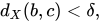
The concept of continuity for functions between metric spaces can be strengthened in various ways by limiting the way \delta depends on \varepsilon and c in the definition above. Intuitively, a function f as above is uniformly continuous if the \delta does not depend on the point c. More precisely, it requires that for every real number \varepsilon >0 there exists \delta >0 such that for every c,b\in X with d_{X}(b,c)<\delta , the inequality d_{Y}(f(b),f(c))<\varepsilon holds. Thus, any uniformly continuous function is continuous. The converse does not hold generally, but holds when the domain space X is compact. Uniformly continuous maps can be defined in the more general situation of uniform spaces.

A function is Hölder continuous with exponent \alpha (a real number) if there is a constant K such that for all b,c\in X, the inequality d_{Y}(f(b),f(c))\leq K\cdot (d_{X}(b,c))^{\alpha } holds. Any Hölder continuous function is uniformly continuous. The particular case \alpha =1 is referred to as Lipschitz continuity. That is, a function is Lipschitz continuous if there is a constant K such that the inequality d_{Y}(f(b),f(c))\leq K\cdot d_{X}(b,c) holds for any b,c\in X. The Lipschitz condition occurs, for example, in the Picard-Lindelöf theorem concerning the solutions of ordinary differential equations.

The graph of a cubic function has no jumps or holes. The function is continuous.

04Continuous functions between topological spaces

Another, more abstract, notion of continuity is the continuity of functions between topological spaces in which there generally is no formal notion of distance, as there is in the case of metric spaces. A topological space is a set X together with a topology on X, which is a set of subsets of X satisfying a few requirements with respect to their unions and intersections that generalize the properties of the open balls in metric spaces while still allowing one to talk about the neighborhoods of a given point. The elements of a topology are called open subsets of X (with respect to the topology).

A function f:X\to Y between two topological spaces X and Y is continuous if for every open set V\subseteq Y, the inverse image f^{-1}(V)=\{x\in X\;|\;f(x)\in V\} is an open subset of X. That is, f is a function between the sets X and Y (not on the elements of the topology T_{X}), but the continuity of f depends on the topologies used on X and Y.

This is equivalent to the condition that the preimages of the closed sets (which are the complements of the open subsets) in Y are closed in X.

An extreme example: if a set X is given the discrete topology (in which every subset is open), all functions f:X\to T to any topological space T are continuous. On the other hand, if X is equipped with the indiscrete topology (in which the only open subsets are the empty set and X) and the space T set is at least T0, then the only continuous functions are the constant functions. Conversely, any function whose codomain is indiscrete is continuous.

Continuity at a point

The translation in the language of neighborhoods of the (\varepsilon ,\delta )-definition of continuity leads to the following definition of the continuity at a point:

A function f:X\to Y is continuous at a point x\in X if and only if, for any neighborhood V of f(x) in Y, there is a neighborhood U of x such that f(U)\subseteq V.

This definition is equivalent to the same statement with neighborhoods restricted to open neighborhoods and can be restated in several ways by using preimages rather than images. One of those ways is the following. As every set that contains a neighborhood is also a neighborhood, and f^{-1}(V)=U is the largest subset U\subseteq X such that f(U)\subseteq V, the above definition may be simplified into:

A function f:X\to Y is continuous at a point x\in X if and only if, for every neighborhood V of f(x) in Y, f^{-1}(V) is a neighborhood of x.

As an open set is a set that is a neighborhood of all its points, a function f:X\to Y is continuous at every point of X if and only if it is a continuous function.

If X and Y are metric spaces, it is equivalent to consider the neighborhood system of open balls centered at x and f(x) instead of all neighborhoods. This gives back the above \varepsilon -\delta definition of continuity in the context of metric spaces. In general topological spaces, there is no notion of nearness or distance. If, however, the target space is a Hausdorff space, it is still true that f is continuous at a if and only if the limit of f as x approaches a is f(a). At an isolated point, every function is continuous.

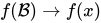
Given x\in X, a map f:X\to Y is continuous at x if and only if whenever {\mathcal {B}} is a filter on X that converges to x in X, which is expressed by writing {\mathcal {B}}\to x, then necessarily f({\mathcal {B}})\to f(x) in Y. If {\mathcal {N}}(x) denotes the neighborhood filter at x then f:X\to Y is continuous at x if and only if f({\mathcal {N}}(x))\to f(x) in Y. Moreover, this happens if and only if the prefilter f({\mathcal {N}}(x)) is a filter base for the neighborhood filter of f(x) in Y.

Alternative definitions

Several equivalent definitions for a topological structure exist; thus, several equivalent ways exist to define a continuous function.

Sequences and nets

In several contexts, the topology of a space is conveniently specified in terms of limit points. This is often accomplished by specifying when a point is the limit of a sequence. Still, for some spaces that are too large in some sense, one specifies also when a point is the limit of more general sets of points indexed by a directed set, known as nets. A function is (Heine-)continuous only if it takes limits of sequences to limits of sequences. In the former case, preservation of limits is also sufficient; in the latter, a function may preserve all limits of sequences yet still fail to be continuous, and preservation of nets is a necessary and sufficient condition.

In detail, a function f:X\to Y is sequentially continuous if whenever a sequence \left(x_{n}\right) in X converges to a limit x, the sequence \left(f\left(x_{n}\right)\right) converges to f(x). Thus, sequentially continuous functions "preserve sequential limits." Every continuous function is sequentially continuous. If X is a first-countable space and countable choice holds, then the converse also holds: any function preserving sequential limits is continuous. In particular, if X is a metric space, sequential continuity and continuity are equivalent. For non-first-countable spaces, sequential continuity might be strictly weaker than continuity. (The spaces for which the two properties are equivalent are called sequential spaces.) This motivates the consideration of nets instead of sequences in general topological spaces. Continuous functions preserve the limits of nets, and this property characterizes continuous functions.

For instance, consider the case of real-valued functions of one real variable:

Theorem, A function f:A\subseteq \mathbb {R} \to \mathbb {R} is continuous at x_{0} if and only if it is sequentially continuous at that point.

Proof

Assume that f:A\subseteq \mathbb {R} \to \mathbb {R} is continuous at x_{0} (in the sense of \varepsilon -\delta continuity). Let \left(x_{n}\right)_{n\geq 1} be a sequence converging at x_{0} (such a sequence always exists, for example, x_{n}=x_{0},{\text{ for all }}n); since f is continuous at x_{0} \forall \varepsilon >0\,\exists \delta _{\varepsilon }>0:0<|x-x_{0}|<\delta _{\varepsilon }\implies |f(x)-f(x_{0})|<\varepsilon .\quad (*) For any such \delta _{\varepsilon } we can find a natural number \nu _{\varepsilon }>0 such that for all n>\nu _{\varepsilon }, |x_{n}-x_{0}|<\delta _{\varepsilon }, since \left(x_{n}\right) converges at x_{0}; combining this with (*) we obtain \forall \varepsilon >0\,\exists \nu _{\varepsilon }>0:\forall n>\nu _{\varepsilon }\quad |f(x_{n})-f(x_{0})|<\varepsilon . Assume on the contrary that f is sequentially continuous and proceed by contradiction: suppose f is not continuous at x_{0} \exists \varepsilon >0:\forall \delta _{\varepsilon }>0,\,\exists x_{\delta _{\varepsilon }}:0<|x_{\delta _{\varepsilon }}-x_{0}|<\delta _{\varepsilon }\implies |f(x_{\delta _{\varepsilon }})-f(x_{0})|>\varepsilon then we can take \delta _{\varepsilon }=1/n,\,\forall n>0 and call the corresponding point x_{\delta _{\varepsilon }}=:x_{n}: in this way we have defined a sequence (x_{n})_{n\geq 1} such that \forall n>0\quad |x_{n}-x_{0}|<{\frac {1}{n}},\quad |f(x_{n})-f(x_{0})|>\varepsilon by construction x_{n}\to x_{0} but f(x_{n})\not \to f(x_{0}), which contradicts the hypothesis of sequential continuity. \blacksquare

Closure operator and interior operator definitions

In terms of the interior and closure operators, we have the following equivalences,

Theorem, Let f:X\to Y be a mapping between topological spaces. Then the following are equivalent.

  1. f is continuous;
  2. for every subset B\subseteq Y, f^{-1}\left(\operatorname {int} _{Y}B\right)\subseteq \operatorname {int} _{X}\left(f^{-1}(B)\right);
  3. for every subset A\subseteq X, f\left(\operatorname {cl} _{X}A\right)\subseteq \operatorname {cl} _{Y}\left(f(A)\right).
Proof

Proof.i ⇒ ii. Fix a subset B of Y. Since \operatorname {int} _{Y}B is open. and f is continuous, f^{-1}(\operatorname {int} _{Y}B) is open in X. As \operatorname {int} _{Y}B\subseteq B, we have f^{-1}(\operatorname {int} _{Y}B)\subseteq f^{-1}(B). By the definition of the interior, \operatorname {int} _{X}\left(f^{-1}(B)\right) is the largest open set contained in f^{-1}(B). Hence f^{-1}(\operatorname {int} _{Y}B)\subseteq \operatorname {int} _{X}\left(f^{-1}(B)\right).

ii ⇒ iii. Fix A\subseteq X and let x\in \operatorname {cl} _{X}A. Suppose to the contrary that f(x)\notin \operatorname {cl} _{Y}\left(f(A)\right), then we may find some open neighbourhood V of f(x) that is disjoint from \operatorname {cl} _{Y}\left(f(A)\right). By ii, f^{-1}(V)=f^{-1}(\operatorname {int} _{Y}V)\subseteq \operatorname {int} _{X}\left(f^{-1}(V)\right), hence f^{-1}(V) is open. Then we have found an open neighbourhood of x that does not intersect \operatorname {cl} _{X}A, contradicting the fact that x\in \operatorname {cl} _{X}A. Hence f\left(\operatorname {cl} _{X}A\right)\subseteq \operatorname {cl} _{Y}\left(f(A)\right).

iii ⇒ i. Let N\subseteq Y be closed. Let M=f^{-1}(N) be the preimage of N. By iii, we have f\left(\operatorname {cl} _{X}M\right)\subseteq \operatorname {cl} _{Y}\left(f(M)\right). Since f(M)=f(f^{-1}(N))\subseteq N, we have further that f\left(\operatorname {cl} _{X}M\right)\subseteq \operatorname {cl} _{Y}N=N. Thus \operatorname {cl} _{X}M\subseteq f^{-1}\left(f(\operatorname {cl} _{X}M)\right)\subseteq f^{-1}(N)=M. Hence M is closed and we are done.

If we declare that a point x is close to a subset A\subseteq X if x\in \operatorname {cl} _{X}A, then this terminology allows for a plain English description of continuity: f is continuous if and only if for every subset A\subseteq X, f maps points that are close to A to points that are close to f(A). Similarly, f is continuous at a fixed given point x\in X if and only if whenever x is close to a subset A\subseteq X, then f(x) is close to f(A).

Instead of specifying topological spaces by their open subsets, any topology on X can alternatively be determined by a closure operator or by an interior operator. Specifically, the map that sends a subset A of a topological space X to its topological closure \operatorname {cl} _{X}A satisfies the Kuratowski closure axioms. Conversely, for any closure operator A\mapsto \operatorname {cl} A there exists a unique topology \tau on X (specifically, \tau :=\{X\setminus \operatorname {cl} A:A\subseteq X\}) such that for every subset A\subseteq X, \operatorname {cl} A is equal to the topological closure \operatorname {cl} _{(X,\tau )}A of A in (X,\tau ). If the sets X and Y are each associated with closure operators (both denoted by \operatorname {cl}) then a map f:X\to Y is continuous if and only if f(\operatorname {cl} A)\subseteq \operatorname {cl} (f(A)) for every subset A\subseteq X.

Similarly, the map that sends a subset A of X to its topological interior \operatorname {int} _{X}A defines an interior operator. Conversely, any interior operator A\mapsto \operatorname {int} A induces a unique topology \tau on X (specifically, \tau :=\{\operatorname {int} A:A\subseteq X\}) such that for every A\subseteq X, \operatorname {int} A is equal to the topological interior \operatorname {int} _{(X,\tau )}A of A in (X,\tau ). If the sets X and Y are each associated with interior operators (both denoted by \operatorname {int}) then a map f:X\to Y is continuous if and only if f^{-1}(\operatorname {int} B)\subseteq \operatorname {int} \left(f^{-1}(B)\right) for every subset B\subseteq Y.

Filters and prefilters

Continuity can also be characterized in terms of filters. A function f:X\to Y is continuous if and only if whenever a filter {\mathcal {B}} on X converges in X to a point x\in X, then the prefilter f({\mathcal {B}}) converges in Y to f(x). This characterization remains true if the word "filter" is replaced by "prefilter".

Properties

If f:X\to Y and g:Y\to Z are continuous, then so is the composition g\circ f:X\to Z. If f:X\to Y is continuous and

The possible topologies on a fixed set X are partially ordered: a topology \tau _{1} is said to be coarser than another topology \tau _{2} (notation: \tau _{1}\subseteq \tau _{2}) if every open subset with respect to \tau _{1} is also open with respect to \tau _{2}. Then, the identity map \operatorname {id} _{X}:\left(X,\tau _{2}\right)\to \left(X,\tau _{1}\right) is continuous if and only if \tau _{1}\subseteq \tau _{2} (see also comparison of topologies). More generally, a continuous function \left(X,\tau _{X}\right)\to \left(Y,\tau _{Y}\right) stays continuous if the topology \tau _{Y} is replaced by a coarser topology and/or \tau _{X} is replaced by a finer topology.

Homeomorphisms

Symmetric to the concept of a continuous map is an open map, for which images of open sets are open. If an open map f has an inverse function, that inverse is continuous, and if a continuous map g has an inverse, that inverse is open. Given a bijective function f between two topological spaces, the inverse function f^{-1} need not be continuous. A bijective continuous function with a continuous inverse function is called a homeomorphism.

If a continuous bijection has as its domain a compact space and its codomain is Hausdorff, then it is a homeomorphism.

Defining topologies via continuous functions

Given a function f:X\to S, where X is a topological space and S is a set (without a specified topology), the final topology on S is defined by letting the open sets of S be those subsets A\subset S for which f^{-1}(A) is open in X. If S has an existing topology, f is continuous with respect to this topology if and only if the existing topology is coarser than the final topology on S. Thus, the final topology is the finest topology on S that makes f continuous. If f is surjective, this topology is canonically identified with the quotient topology under the equivalence relation defined by f.

Dually, for a function f from a set S to a topological space X, the initial topology on S is defined by designating as an open set every subset A\subset S such that A=f^{-1}(U) for some open subset U of X. If S has an existing topology, f is continuous with respect to this topology if and only if the existing topology is finer than the initial topology on S. Thus, the initial topology is the coarsest topology on S that makes f continuous. If f is injective, this topology is canonically identified with the subspace topology of S, viewed as a subset of X.

A topology on a set S is uniquely determined by the class of all continuous functions S\to X into all topological spaces X. Dually, a similar idea can be applied to maps X\to S.

The graph of a continuous rational function. The function is not defined for The vertical and horizontal lines are asymptotes.
The sinc and the cos functions
Watch videos about Continuous functionExplainers and documentaries on YouTube (opens in a new tab)

Sources and credits

This article is adapted from the Wikipedia article Continuous function, written by its contributors and licensed under CC BY-SA 4.0. Fathomly has changed the layout, removed citation markers, navigation and maintenance notices, and adjusted punctuation. This adapted version is shared under the same license. For references, see the original article.

Images, from Wikimedia Commons:

Fathomly is not affiliated with or endorsed by the Wikimedia Foundation. Spotted a problem? Tell us.