Encyclopedia

Heaviside step function

Indicator function of positive numbers

Wikipedia contributorsAdapted for Fathomly · View authors

5 min read
Source updated September 15, 2026

The Heaviside step function, or the unit step function, usually denoted by H or θ (but sometimes u, 1 or 𝟙), is a step function named after Oliver Heaviside, the value of which is zero for negative arguments and one for positive arguments. Different conventions concerning the value H(0) are in use. It is an example of the general class of step functions, all of which can be represented as linear combinations of translations of this one.

The function was originally developed in operational calculus for the solution of differential equations, where it represents a signal that switches on at a specified time and stays switched on indefinitely. Heaviside developed the operational calculus as a tool in the analysis of telegraphic communications and represented the function as 1.

01Formulation

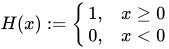
Taking the convention that H(0) = 1, the Heaviside function may be defined as:

A piecewise function: $H(x):={\begin{cases}1,&x\geq 0\\0,&x<0\end{cases}}$
Using the Iverson bracket notation: $H(x):=[x\geq 0]$
An indicator function: $H(x):=\mathbf {1} _{x\geq 0}=\mathbf {1} _{\mathbb {R} _{+}}(x)$

For the alternative convention that H(0) = ⁠1/2⁠, it may be expressed as:

A piecewise function: $H(x):={\begin{cases}1,&x>0\\{\frac {1}{2}},&x=0\\0,&x<0\end{cases}}$
A linear transformation of the sign function: $H(x):={\frac {1}{2}}\left({\mbox{sgn}}\,x+1\right)$
The arithmetic mean of two Iverson brackets: $H(x):={\frac {[x\geq 0]+[x>0]}{2}}$
A one-sided limit of the two-argument arctangent: $H(x)=:\lim _{\epsilon \to 0^{+}}{\frac {{\mbox{atan2}}(\epsilon ,-x)}{\pi }}$
A hyperfunction: $H(x)=:\left(1-{\frac {1}{2\pi i}}\log z,\ -{\frac {1}{2\pi i}}\log z\right)$ Or equivalently: $H(x)=:\left(-{\frac {\log -z}{2\pi i}},-{\frac {\log -z}{2\pi i}}\right),$ where log z is the principal value of the complex logarithm of z.

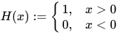
Other definitions that are undefined at H(0) include:

A piecewise function: $H(x):={\begin{cases}1,&x>0\\0,&x<0\end{cases}}$
The derivative of the ramp function: $H(x):={\frac {d}{dx}}\max\{x,0\}\quad {\mbox{for }}x\neq 0$
Expressed in terms of the absolute value function, such as: $H(x)={\frac {1}{2}}+{\frac {|x|}{2x}}$

02Relationship with Dirac delta function

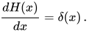
The Dirac delta function is the weak derivative of the Heaviside function: $\delta (x)={\frac {d}{dx}}\ H(x),$ Hence the Heaviside function can be considered to be the integral of the Dirac delta function. This is sometimes written as: $H(x):=\int _{-\infty }^{x}\delta (s)\,ds,$ although this expansion may not hold (or even make sense) for x = 0, depending on which formalism one uses to give meaning to integrals involving δ. In this context, the Heaviside function is the cumulative distribution function of a random variable that is almost surely 0. (See Constant random variable.)

03Analytic approximations

Approximations to the Heaviside step function are of use in biochemistry and neuroscience, where logistic approximations of step functions (such as the Hill and the Michaelis-Menten equations) may be used to approximate binary cellular switches in response to chemical signals.

For a smooth approximation to the step function, one can use the logistic function: $H(x)\approx {\tfrac {1}{2}}+{\tfrac {1}{2}}\tanh kx={\frac {1}{1+e^{-2kx}}},$ where a larger k corresponds to a sharper transition at x = 0.

If we take H(0) = ⁠1/2⁠, equality holds in the limit: $H(x)=\lim _{k\to \infty }{\tfrac {1}{2}}(1+\tanh kx)=\lim _{k\to \infty }{\frac {1}{1+e^{-2kx}}}.$

There are many other smooth, analytic approximations to the step function. Among the possibilities are: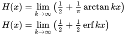 ${\begin{aligned}H(x)&=\lim _{k\to \infty }\left({\tfrac {1}{2}}+{\tfrac {1}{\pi }}\arctan kx\right)\\H(x)&=\lim _{k\to \infty }\left({\tfrac {1}{2}}+{\tfrac {1}{2}}\operatorname {erf} kx\right)\end{aligned}}$ These limits hold pointwise and in the sense of distributions. In general, however, pointwise convergence need not imply distributional convergence, and vice versa distributional convergence need not imply pointwise convergence. (However, if all members of a pointwise convergent sequence of functions are uniformly bounded by some "nice" function, then convergence holds in the sense of distributions too.)

One could also use a scaled and shifted Sigmoid function.

In general, any cumulative distribution function of a continuous probability distribution that is peaked around zero and has a parameter that controls for variance can serve as an approximation, in the limit as the variance approaches zero. For example, all three of the above approximations are cumulative distribution functions of common probability distributions: the logistic, Cauchy and normal distributions, respectively.

04Non-analytic approximations

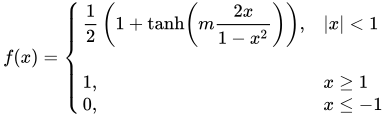
Approximations to the Heaviside step function could be made through Smooth transition function like $1\leq m\to \infty$ : ${\begin{aligned}f(x)&={\begin{cases}{\displaystyle {\frac {1}{2}}\left(1+\tanh \left(m{\frac {2x}{1-x^{2}}}\right)\right)},&|x|<1\\\\1,&x\geq 1\\0,&x\leq -1\end{cases}}\end{aligned}}$

05Integral representations

Often an integral representation of the Heaviside step function is useful: ${\begin{aligned}H(x)&=\lim _{\varepsilon \to 0^{+}}-{\frac {1}{2\pi i}}\int _{-\infty }^{\infty }{\frac {1}{\tau +i\varepsilon }}e^{-ix\tau }d\tau \\&=\lim _{\varepsilon \to 0^{+}}\ {\frac {1}{2\pi i}}\int _{-\infty }^{\infty }{\frac {1}{\tau -i\varepsilon }}e^{ix\tau }d\tau ,\end{aligned}}$ where the second representation is easy to deduce from the first, given that the step function is real and thus is its own complex conjugate.

06Zero argument

Since H is usually used in integration, and the value of a function at a single point does not affect its integral, it rarely matters what particular value is chosen of H(0). Indeed when H is considered as a distribution or an element of L^∞ (see L^p space) it does not even make sense to talk of a value at zero, since such objects are only defined almost everywhere. If using some analytic approximation (as in the examples above) then often whatever happens to be the relevant limit at zero is used.

There exist various reasons for choosing a particular value.

H(0) = ⁠1/2⁠ is often used since the graph then has rotational symmetry; put another way, H − ⁠1/2⁠ is then an odd function. In this case the following relation with the sign function holds for all x: $H(x)={\tfrac {1}{2}}(1+\operatorname {sgn} x).$ Also, $\forall x,\ H(x)+H(-x)=1$ .
H(0) = 1 is used when H needs to be right-continuous. For instance cumulative distribution functions are usually taken to be right continuous, as are functions integrated against in Lebesgue-Stieltjes integration. In this case H is the indicator function of a closed semi-infinite interval: $H(x)=\mathbf {1} _{[0,\infty )}(x).$ The corresponding probability distribution is the degenerate distribution.
H(0) = 0 is used when H needs to be left-continuous. In this case H is an indicator function of an open semi-infinite interval: $H(x)=\mathbf {1} _{(0,\infty )}(x).$
In functional-analysis contexts from optimization and game theory, it is often useful to define the Heaviside function as a set-valued function to preserve the continuity of the limiting functions and ensure the existence of certain solutions. In these cases, the Heaviside function returns a whole interval of possible solutions, H(0) = [0,1].

07Discrete form

An alternative form of the unit step, defined instead as a function $H:\mathbb {Z} \rightarrow \mathbb {R}$ (that is, taking in a discrete variable n), is: $H[n]={\begin{cases}0,&n<0,\\1,&n\geq 0,\end{cases}}$ Or using the half-maximum convention: $H[n]={\begin{cases}0,&n<0,\\{\tfrac {1}{2}},&n=0,\\1,&n>0,\end{cases}}$ where n is an integer. If n is an integer, then n < 0 must imply that n ≤ −1, while n > 0 must imply that the function attains unity at n = 1. Therefore the "step function" exhibits ramp-like behavior over the domain of [−1, 1], and cannot authentically be a step function, using the half-maximum convention.

Unlike the continuous case, the definition of H[0] is significant.

The discrete-time unit impulse is the first difference of the discrete-time step: $\delta [n]=H[n]-H[n-1].$ This function is the cumulative summation of the Kronecker delta: $H[n]=\sum _{k=-\infty }^{n}\delta [k],$ where ${\textstyle \delta [k]=\delta _{k,0}$ is the discrete unit impulse function.

08Antiderivative and derivative

The ramp function is an antiderivative of the Heaviside step function: $\int _{-\infty }^{x}H(\xi )\,d\xi =xH(x)=\max\{0,x\}\,.$ The distributional derivative of the Heaviside step function is the Dirac delta function: ${\frac {dH(x)}{dx}}=\delta (x)\,.$

09Fourier transform

The Fourier transform of the Heaviside step function is a distribution. Using one choice of constants for the definition of the Fourier transform we have ${\hat {H}}(s)=\lim _{N\to \infty }\int _{-N}^{N}e^{-2\pi ixs}H(x)\,dx={\frac {1}{2}}\left(\delta (s)-{\frac {i}{\pi }}\operatorname {p.v.} {\frac {1}{s}}\right).$ Here p.v.⁠1/s⁠ is the distribution that takes a test function φ to the Cauchy principal value of $\textstyle \int _{-\infty }^{\infty }{\frac {\varphi (s)}{s}}\,ds$ . The limit appearing in the integral is also taken in the sense of (tempered) distributions.

10Unilateral Laplace transform

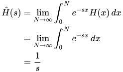
The Laplace transform of the Heaviside step function is a meromorphic function. Using the unilateral Laplace transform we have: ${\begin{aligned}{\hat {H}}(s)&=\lim _{N\to \infty }\int _{0}^{N}e^{-sx}H(x)\,dx\\&=\lim _{N\to \infty }\int _{0}^{N}e^{-sx}\,dx\\&={\frac {1}{s}}\end{aligned}}$

When the bilateral transform is used, the integral can be split in two parts and the result will be the same.

Watch videos about Heaviside step functionExplainers and documentaries on YouTube (opens in a new tab)

Sources and credits

This article is adapted from the Wikipedia article “Heaviside step function”, written by its contributors and licensed under CC BY-SA 4.0. Fathomly has changed the layout, removed citation markers, navigation and maintenance notices, and adjusted punctuation. This adapted version is shared under the same license. For references, see the original article.

Images, from Wikimedia Commons:

Dirac distribution CDF.svg by Omegatron, CC BY-SA 3.0
Step function approximation.png by Hersle, CC BY-SA 4.0

Fathomly is not affiliated with or endorsed by the Wikimedia Foundation. Spotted a problem? Tell us.