Encyclopedia

Poisson bracket

Operation in Hamiltonian mechanics

Wikipedia contributorsAdapted for Fathomly · View authors

7 min read
Source updated April 2, 2026

Image credit is listed at the end of this article.

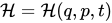
In mathematics and classical mechanics, the Poisson bracket is an important binary operation in Hamiltonian mechanics, playing a central role in Hamilton's equations of motion, which govern the time evolution of a Hamiltonian dynamical system. The Poisson bracket also distinguishes a certain class of coordinate transformations, called canonical transformations, which map canonical coordinate systems into other canonical coordinate systems. A "canonical coordinate system" consists of canonical position and momentum variables (below symbolized by $q_{i}$ and $p_{i}$ , respectively) that satisfy canonical Poisson bracket relations. The set of possible canonical transformations is always very rich. For instance, it is often possible to choose the Hamiltonian itself ${\mathcal {H}}={\mathcal {H}}(q,p,t)$ as one of the new canonical momentum coordinates.

In a more general sense, the Poisson bracket is used to define a Poisson algebra, of which the algebra of functions on a Poisson manifold is a special case. There are other general examples, as well: it occurs in the theory of Lie algebras, where the tensor algebra of a Lie algebra forms a Poisson algebra; a detailed construction of how this comes about is given in the universal enveloping algebra article. Quantum deformations of the universal enveloping algebra lead to the notion of quantum groups.

All of these objects are named in honor of French mathematician Siméon Denis Poisson. He introduced the Poisson bracket in his 1809 treatise on mechanics.

01Properties

Given two functions f and g that depend on phase space and time, their Poisson bracket $\{f,g\}$ is another function that depends on phase space and time. The following rules hold for any three functions $f,\,g,\,h$ of phase space and time:

Anticommutativity: $\{f,g\}=-\{g,f\}$
Bilinearity: $\{af+bg,h\}=a\{f,h\}+b\{g,h\},$ $\{h,af+bg\}=a\{h,f\}+b\{h,g\},\quad a,b\in \mathbb {R}$
Leibniz's rule: $\{fg,h\}=\{f,h\}g+f\{g,h\}$
Jacobi identity: $\{f,\{g,h\}\}+\{g,\{h,f\}\}+\{h,\{f,g\}\}=0$

Also, if a function $k$ is constant over phase space (but may depend on time), then $\{f,\,k\}=0$ for any $f$ .

02Definition in canonical coordinates

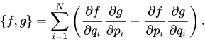
In canonical coordinates (also known as Darboux coordinates) $(q_{i},\,p_{i})$ on the phase space, given two functions $f(p_{i},\,q_{i},t)$ and $g(p_{i},\,q_{i},t)$ , the Poisson bracket takes the form $\{f,g\}=\sum _{i=1}^{N}\left({\frac {\partial f}{\partial q_{i}}}{\frac {\partial g}{\partial p_{i}}}-{\frac {\partial f}{\partial p_{i}}}{\frac {\partial g}{\partial q_{i}}}\right).$

The Poisson brackets of the canonical coordinates are ${\begin{aligned}\{q_{k},q_{l}\}&=\sum _{i=1}^{N}\left({\frac {\partial q_{k}}{\partial q_{i}}}{\frac {\partial q_{l}}{\partial p_{i}}}-{\frac {\partial q_{k}}{\partial p_{i}}}{\frac {\partial q_{l}}{\partial q_{i}}}\right)=\sum _{i=1}^{N}\left(\delta _{ki}\cdot 0-0\cdot \delta _{li}\right)=0,\\\{p_{k},p_{l}\}&=\sum _{i=1}^{N}\left({\frac {\partial p_{k}}{\partial q_{i}}}{\frac {\partial p_{l}}{\partial p_{i}}}-{\frac {\partial p_{k}}{\partial p_{i}}}{\frac {\partial p_{l}}{\partial q_{i}}}\right)=\sum _{i=1}^{N}\left(0\cdot \delta _{li}-\delta _{ki}\cdot 0\right)=0,\\\{q_{k},p_{l}\}&=\sum _{i=1}^{N}\left({\frac {\partial q_{k}}{\partial q_{i}}}{\frac {\partial p_{l}}{\partial p_{i}}}-{\frac {\partial q_{k}}{\partial p_{i}}}{\frac {\partial p_{l}}{\partial q_{i}}}\right)=\sum _{i=1}^{N}\left(\delta _{ki}\cdot \delta _{li}-0\cdot 0\right)=\delta _{kl},\end{aligned}}$ where $\delta _{ij}$ is the Kronecker delta.

03Hamilton's equations of motion

Hamilton's equations of motion have an equivalent expression in terms of the Poisson bracket. This may be most directly demonstrated in an explicit coordinate frame. Suppose that $f(p,q,t)$ is a function on the solution's trajectory-manifold. Then from the multivariable chain rule, ${\frac {d}{dt}}f(p,q,t)={\frac {\partial f}{\partial q}}{\frac {dq}{dt}}+{\frac {\partial f}{\partial p}}{\frac {dp}{dt}}+{\frac {\partial f}{\partial t}}.$

Further, one may take $p=p(t)$ and $q=q(t)$ to be solutions to Hamilton's equations; that is, ${\begin{aligned}{\frac {dq}{dt}}&={\frac {\partial {\mathcal {H}}}{\partial p}}=\{q,{\mathcal {H}}\},\\{\frac {dp}{dt}}&=-{\frac {\partial {\mathcal {H}}}{\partial q}}=\{p,{\mathcal {H}}\}.\end{aligned}}$

Then ${\begin{aligned}{\frac {d}{dt}}f(p,q,t)&={\frac {\partial f}{\partial q}}{\frac {\partial {\mathcal {H}}}{\partial p}}-{\frac {\partial f}{\partial p}}{\frac {\partial {\mathcal {H}}}{\partial q}}+{\frac {\partial f}{\partial t}}\\&=\{f,{\mathcal {H}}\}+{\frac {\partial f}{\partial t}}~.\end{aligned}}$

Thus, the time evolution of a function $f$ on a symplectic manifold can be given as a one-parameter family of symplectomorphisms (i.e., canonical transformations, area-preserving diffeomorphisms), with the time $t$ being the parameter: Hamiltonian motion is a canonical transformation generated by the Hamiltonian. That is, Poisson brackets are preserved in it, so that any time $t$ in the solution to Hamilton's equations, $q(t)=\exp(-t\{{\mathcal {H}},\cdot \})q(0),\quad p(t)=\exp(-t\{{\mathcal {H}},\cdot \})p(0),$ can serve as the bracket coordinates. Poisson brackets are canonical invariants.

Dropping the coordinates, ${\frac {d}{dt}}f=\left({\frac {\partial }{\partial t}}-\{{\mathcal {H}},\cdot \}\right)f.$

The operator in the convective part of the derivative, $i{\hat {L}}=-\{{\mathcal {H}},\cdot \}$ , is sometimes referred to as the Liouvillian (see Liouville's theorem (Hamiltonian)).

04Poisson matrix in canonical transformations

The concept of Poisson brackets can be expanded to that of matrices by defining the Poisson matrix.

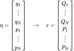
Consider the following canonical transformation: $\eta ={\begin{bmatrix}q_{1}\\\vdots \\q_{N}\\p_{1}\\\vdots \\p_{N}\\\end{bmatrix}}\quad \rightarrow \quad \varepsilon ={\begin{bmatrix}Q_{1}\\\vdots \\Q_{N}\\P_{1}\\\vdots \\P_{N}\\\end{bmatrix}}$ Defining ${\textstyle M:={\frac {\partial (\mathbf {Q} ,\mathbf {P} )}{\partial (\mathbf {q} ,\mathbf {p} )}}$ , the Poisson matrix is defined as ${\textstyle {\mathcal {P}}(\varepsilon )=MJM^{T}$ , where $J$ is the symplectic matrix under the same conventions used to order the set of coordinates. It follows from the definition that: ${\mathcal {P}}_{ij}(\varepsilon )=[MJM^{T}]_{ij}=\sum _{k=1}^{N}\left({\frac {\partial \varepsilon _{i}}{\partial \eta _{k}}}{\frac {\partial \varepsilon _{j}}{\partial \eta _{N+k}}}-{\frac {\partial \varepsilon _{i}}{\partial \eta _{N+k}}}{\frac {\partial \varepsilon _{j}}{\partial \eta _{k}}}\right)=\sum _{k=1}^{N}\left({\frac {\partial \varepsilon _{i}}{\partial q_{k}}}{\frac {\partial \varepsilon _{j}}{\partial p_{k}}}-{\frac {\partial \varepsilon _{i}}{\partial p_{k}}}{\frac {\partial \varepsilon _{j}}{\partial q_{k}}}\right)=\{\varepsilon _{i},\varepsilon _{j}\}_{\eta }.$

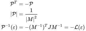
The Poisson matrix satisfies the following known properties: ${\begin{aligned}{\mathcal {P}}^{T}&=-{\mathcal {P}}\\|{\mathcal {P}}|&={\frac {1}{|M|^{2}}}\\{\mathcal {P}}^{-1}(\varepsilon )&=-(M^{-1})^{T}JM^{-1}=-{\mathcal {L}}(\varepsilon )\\\end{aligned}}$

where the ${\textstyle {\mathcal {L}}(\varepsilon )$ is known as a Lagrange matrix and whose elements correspond to Lagrange brackets. The last identity can also be stated as the following: $\sum _{k=1}^{2N}\{\eta _{i},\eta _{k}\}[\eta _{k},\eta _{j}]=-\delta _{ij}$ Note that the summation here involves generalized coordinates as well as generalized momentum.

The invariance of Poisson bracket can be expressed as: ${\textstyle \{\varepsilon _{i},\varepsilon _{j}\}_{\eta }=\{\varepsilon _{i},\varepsilon _{j}\}_{\varepsilon }=J_{ij}$ , which directly leads to the symplectic condition: ${\textstyle MJM^{T}=J$ .

05Constants of motion

An integrable system will have constants of motion in addition to the energy. Such constants of motion will commute with the Hamiltonian under the Poisson bracket. Suppose some function $f(p,q)$ is a constant of motion. This implies that if $p(t),q(t)$ is a trajectory or solution to Hamilton's equations of motion, then along that trajectory: $0={\frac {df}{dt}}$ Where, as above, the intermediate step follows by applying the equations of motion and we assume that $f$ does not explicitly depend on time. This equation is known as the Liouville equation. The content of Liouville's theorem is that the time evolution of a measure given by a distribution function $f$ is given by the above equation.

If the Poisson bracket of $f$ and $g$ vanishes ( $\{f,g\}=0$ ), then $f$ and $g$ are said to be in involution. In order for a Hamiltonian system to be completely integrable, $n$ independent constants of motion must be in mutual involution, where $n$ is the number of degrees of freedom.

Furthermore, according to Poisson's Theorem, if two quantities $A$ and $B$ are explicitly time independent ( $A(p,q),B(p,q)$ ) constants of motion, so is their Poisson bracket $\{A,\,B\}$ . This follows from the Jacobi identity (see section below). Poisson's Theorem does not always supply a useful result, however, since the number of possible constants of motion is limited ( $2n-1$ for a system with $n$ degrees of freedom), and so the result may be trivial (a constant, or a function of $A$ and $B$ .)

06The Poisson bracket in coordinate-free language

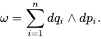
Let $M$ be a symplectic manifold, that is, a manifold equipped with a symplectic form: a 2-form $\omega$ which is both closed (i.e., its exterior derivative $d\omega$ vanishes) and non-degenerate. For example, in the treatment above, take $M$ to be $\mathbb {R} ^{2n}$ and take $\omega =\sum _{i=1}^{n}dq_{i}\wedge dp_{i}.$

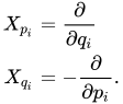
If $\iota _{v}\omega$ is the interior product or contraction operation defined by $(\iota _{v}\omega )(u)=\omega (v,\,u)$ , then non-degeneracy is equivalent to saying that for every one-form $\alpha$ there is a unique vector field $\Omega _{\alpha }$ such that $\iota _{\Omega _{\alpha }}\omega =\alpha$ . Alternatively, $\Omega _{dH}=\omega ^{-1}(dH)$ . Then if $H$ is a smooth function on $M$ , the Hamiltonian vector field $X_{H}$ can be defined to be $\Omega _{dH}$ . It is easy to see that ${\begin{aligned}X_{p_{i}}&={\frac {\partial }{\partial q_{i}}}\\X_{q_{i}}&=-{\frac {\partial }{\partial p_{i}}}.\end{aligned}}$

The Poisson bracket $\ \{\cdot ,\,\cdot \}$ on (M, ω) is a bilinear operation on differentiable functions, defined by $\{f,\,g\}\;=\;\omega (X_{f},\,X_{g})$ ; the Poisson bracket of two functions on M is itself a function on M. The Poisson bracket is antisymmetric because: $\{f,g\}=\omega (X_{f},X_{g})=-\omega (X_{g},X_{f})=-\{g,f\}.$

Furthermore,

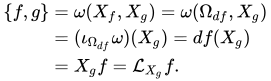
{\begin{aligned}\{f,g\}&=\omega (X_{f},X_{g})=\omega (\Omega _{df},X_{g})\\&=(\iota _{\Omega _{df}}\omega )(X_{g})=df(X_{g})\\&=X_{g}f={\mathcal {L}}_{X_{g}}f.\end{aligned}}

Here X_gf denotes the vector field X_g applied to the function f as a directional derivative, and ${\mathcal {L}}_{X_{g}}f$ denotes the (entirely equivalent) Lie derivative of the function f.

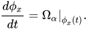
If α is an arbitrary one-form on M, the vector field Ω_α generates (at least locally) a flow $\phi _{x}(t)$ satisfying the boundary condition $\phi _{x}(0)=x$ and the first-order differential equation ${\frac {d\phi _{x}}{dt}}=\left.\Omega _{\alpha }\right|_{\phi _{x}(t)}.$

The $\phi _{x}(t)$ will be symplectomorphisms (canonical transformations) for every t as a function of x if and only if ${\mathcal {L}}_{\Omega _{\alpha }}\omega \;=\;0$ ; when this is true, Ω_α is called a symplectic vector field. Recalling Cartan's identity ${\mathcal {L}}_{X}\omega \;=\;d(\iota _{X}\omega )\,+\,\iota _{X}d\omega$ and dω = 0, it follows that ${\mathcal {L}}_{\Omega _{\alpha }}\omega \;=\;d\left(\iota _{\Omega _{\alpha }}\omega \right)\;=\;d\alpha$ . Therefore, Ω_α is a symplectic vector field if and only if α is a closed form. Since $d(df)\;=\;d^{2}f\;=\;0$ , it follows that every Hamiltonian vector field X_f is a symplectic vector field, and that the Hamiltonian flow consists of canonical transformations. From (1) above, under the Hamiltonian flow $X_{\mathcal {H}}$ , ${\frac {d}{dt}}f(\phi _{x}(t))=X_{\mathcal {H}}f=\{f,{\mathcal {H}}\}.$

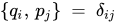
This is a fundamental result in Hamiltonian mechanics, governing the time evolution of functions defined on phase space. As noted above, when $\{f,{\mathcal {H}}\}=0$ , f is a constant of motion of the system. In addition, in canonical coordinates (with $\{p_{i},\,p_{j}\}\;=\;\{q_{i},q_{j}\}\;=\;0$ and $\{q_{i},\,p_{j}\}\;=\;\delta _{ij}$ ), Hamilton's equations for the time evolution of the system follow immediately from this formula.

It also follows from (1) that the Poisson bracket is a derivation; that is, it satisfies a non-commutative version of Leibniz's product rule:

\{fg,h\}=f\{g,h\}+g\{f,h\},

and

\{f,gh\}=g\{f,h\}+h\{f,g\}.

The Poisson bracket is intimately connected to the Lie bracket of the Hamiltonian vector fields. Because the Lie derivative is a derivation, ${\mathcal {L}}_{v}\iota _{u}\omega =\iota _{{\mathcal {L}}_{v}u}\omega +\iota _{u}{\mathcal {L}}_{v}\omega =\iota _{[v,u]}\omega +\iota _{u}{\mathcal {L}}_{v}\omega .$

Thus if v and u are symplectic, using ${\mathcal {L}}_{v}\omega =0={\mathcal {L}}_{u}\omega$ , Cartan's identity, and the fact that $\iota _{u}\omega$ is a closed form, $\iota _{[v,u]}\omega ={\mathcal {L}}_{v}\iota _{u}\omega =d(\iota _{v}\iota _{u}\omega )+\iota _{v}d(\iota _{u}\omega )=d(\iota _{v}\iota _{u}\omega )=d(\omega (u,v)).$

It follows that $[v,u]=X_{\omega (u,v)}$ , so that

[X_{f},X_{g}]=X_{\omega (X_{g},X_{f})}=-X_{\omega (X_{f},X_{g})}=-X_{\{f,g\}}.

Thus, the Poisson bracket on functions corresponds to the Lie bracket of the associated Hamiltonian vector fields. We have also shown that the Lie bracket of two symplectic vector fields is a Hamiltonian vector field and hence is also symplectic. In the language of abstract algebra, the symplectic vector fields form a subalgebra of the Lie algebra of smooth vector fields on M, and the Hamiltonian vector fields form an ideal of this subalgebra. The symplectic vector fields are the Lie algebra of the (infinite-dimensional) Lie group of symplectomorphisms of M.

It is widely asserted that the Jacobi identity for the Poisson bracket, $\{f,\{g,h\}\}+\{g,\{h,f\}\}+\{h,\{f,g\}\}=0$ follows from the corresponding identity for the Lie bracket of vector fields, but this is true only up to a locally constant function. However, to prove the Jacobi identity for the Poisson bracket, it is sufficient to show that: $\operatorname {ad} _{\{g,f\}}=\operatorname {ad} _{-\{f,g\}}=[\operatorname {ad} _{f},\operatorname {ad} _{g}]$ where the operator $\operatorname {ad} _{g}$ on smooth functions on M is defined by $\operatorname {ad} _{g}(\cdot )\;=\;\{\cdot ,\,g\}$ and the bracket on the right-hand side is the commutator of operators, $[\operatorname {A} ,\,\operatorname {B} ]\;=\;\operatorname {A} \operatorname {B} -\operatorname {B} \operatorname {A}$ . By (1), the operator $\operatorname {ad} _{g}$ is equal to the operator X_g. The proof of the Jacobi identity follows from (3) because, up to the factor of -1, the Lie bracket of vector fields is just their commutator as differential operators.

The algebra of smooth functions on M, together with the Poisson bracket forms a Poisson algebra, because it is a Lie algebra under the Poisson bracket, which additionally satisfies Leibniz's rule (2). We have shown that every symplectic manifold is a Poisson manifold, that is a manifold with a "curly-bracket" operator on smooth functions such that the smooth functions form a Poisson algebra. However, not every Poisson manifold arises in this way, because Poisson manifolds allow for degeneracy which cannot arise in the symplectic case.

07A result on conjugate momenta

Given a smooth vector field $X$ on the configuration space, let $P_{X}$ be its conjugate momentum. The conjugate momentum mapping is a Lie algebra anti-homomorphism from the Lie bracket to the Poisson bracket: $\{P_{X},P_{Y}\}=-P_{[X,Y]}.$

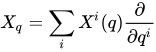
This important result is worth a short proof. Write a vector field $X$ at point $q$ in the configuration space as $X_{q}=\sum _{i}X^{i}(q){\frac {\partial }{\partial q^{i}}}$ where ${\textstyle {\frac {\partial }{\partial q^{i}}}$ is the local coordinate frame. The conjugate momentum to $X$ has the expression $P_{X}(q,p)=\sum _{i}X^{i}(q)\;p_{i}$ where the $p_{i}$ are the momentum functions conjugate to the coordinates. One then has, for a point $(q,p)$ in the phase space, ${\begin{aligned}\{P_{X},P_{Y}\}(q,p)&=\sum _{i}\sum _{j}\left\{X^{i}(q)\;p_{i},Y^{j}(q)\;p_{j}\right\}\\&=\sum _{ij}p_{i}Y^{j}(q){\frac {\partial X^{i}}{\partial q^{j}}}-p_{j}X^{i}(q){\frac {\partial Y^{j}}{\partial q^{i}}}\\&=-\sum _{i}p_{i}\;[X,Y]^{i}(q)\\&=-P_{[X,Y]}(q,p).\end{aligned}}$

The above holds for all $(q,p)$ , giving the desired result.

08Quantization

Poisson brackets deform to Moyal brackets upon quantization, that is, they generalize to a different Lie algebra, the Moyal algebra, or, equivalently in Hilbert space, quantum commutators. The Wigner-İnönü group contraction of these (the classical limit, ħ → 0) yields the above Lie algebra.

To state this more explicitly and precisely, the universal enveloping algebra of the Heisenberg algebra is the Weyl algebra (modulo the relation that the center be the unit). The Moyal product is then a special case of the star product on the algebra of symbols. An explicit definition of the algebra of symbols, and the star product is given in the article on the universal enveloping algebra.

Watch videos about Poisson bracketExplainers and documentaries on YouTube (opens in a new tab)

Sources and credits

This article is adapted from the Wikipedia article “Poisson bracket”, written by its contributors and licensed under CC BY-SA 4.0. Fathomly has changed the layout, removed citation markers, navigation and maintenance notices, and adjusted punctuation. This adapted version is shared under the same license. For references, see the original article.

Images, from Wikimedia Commons:

Simeon Poisson crop.jpg by François-Séraphin Delpech / After Nicolas Eustache Maurin, Public domain

Fathomly is not affiliated with or endorsed by the Wikimedia Foundation. Spotted a problem? Tell us.