Encyclopedia

Linear form

Linear map from a vector space to its field of scalars

Wikipedia contributorsAdapted for Fathomly · View authors

11 min read
Source updated September 14, 2026

In mathematics, a linear form (also known as a linear functional, a one-form, or a covector) is a linear map from a vector space to its field of scalars (often, the real numbers or the complex numbers).

If V is a vector space over a field k, the set of all linear functionals from V to k is itself a vector space over k with addition and scalar multiplication defined pointwise. This space is called the dual space of V, or sometimes the algebraic dual space, when a topological dual space is also considered. It is often denoted Hom(V, k), or, when the field k is understood, $V^{*}$ ; other notations are also used, such as $V'$ , $V^{\#}$ or $V^{\vee }.$ When vectors are represented by column vectors (as is common when a basis is fixed), then linear functionals are represented as row vectors, and their values on specific vectors are given by matrix products (with the row vector on the left).

01Examples

The constant zero function, mapping every vector to zero, is trivially a linear functional. Every other linear functional (such as the ones below) is surjective (that is, its range is all of k).

Indexing into a vector: The second element of a three-vector is given by the one-form $[0,1,0].$ That is, the second element of $[x,y,z]$ is $[0,1,0]\cdot [x,y,z]=y.$
Mean: The mean element of an $n$ -vector is given by the one-form $\left[1/n,1/n,\ldots ,1/n\right].$ That is, $\operatorname {mean} (v)=\left[1/n,1/n,\ldots ,1/n\right]\cdot v.$
Sampling: Sampling with a kernel can be considered a one-form, where the one-form is the kernel shifted to the appropriate location.
Net present value of a net cash flow, $R(t),$ is given by the one-form $w(t)=(1+i)^{-t}$ where $i$ is the discount rate. That is, $\mathrm {NPV} (R(t))=\langle w,R\rangle =\int _{t=0}^{\infty }{\frac {R(t)}{(1+i)^{t}}}\,dt.$

Linear functionals in Rⁿ

Suppose that vectors in the real coordinate space $\mathbb {R} ^{n}$ are represented as column vectors $\mathbf {x} ={\begin{bmatrix}x_{1}\\\vdots \\x_{n}\end{bmatrix}}.$

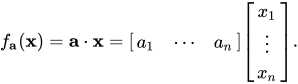
For each row vector $\mathbf {a} ={\begin{bmatrix}a_{1}&\cdots &a_{n}\end{bmatrix}}$ there is a linear functional $f_{\mathbf {a} }$ defined by $f_{\mathbf {a} }(\mathbf {x} )=a_{1}x_{1}+\cdots +a_{n}x_{n},$ and each linear functional can be expressed in this form.

This can be interpreted as either the matrix product or the dot product of the row vector $\mathbf {a}$ and the column vector $\mathbf {x}$ : $f_{\mathbf {a} }(\mathbf {x} )=\mathbf {a} \cdot \mathbf {x} ={\begin{bmatrix}a_{1}&\cdots &a_{n}\end{bmatrix}}{\begin{bmatrix}x_{1}\\\vdots \\x_{n}\end{bmatrix}}.$

Trace of a square matrix

The trace $\operatorname {tr} (A)$ of a square matrix $A$ is the sum of all elements on its main diagonal. Matrices can be multiplied by scalars and two matrices of the same dimension can be added together; these operations make a vector space from the set of all $n\times n$ matrices. The trace is a linear functional on this space because $\operatorname {tr} (sA)=s\operatorname {tr} (A)$ and $\operatorname {tr} (A+B)=\operatorname {tr} (A)+\operatorname {tr} (B)$ for all scalars $s$ and all $n\times n$ matrices $A{\text{ and }}B.$

(Definite) integration

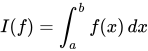
Linear functionals first appeared in functional analysis, the study of vector spaces of functions. A typical example of a linear functional is integration: the linear transformation defined by the Riemann integral $I(f)=\int _{a}^{b}f(x)\,dx$ is a linear functional from the vector space $C[a,b]$ of continuous functions on the interval $[a,b]$ to the real numbers. The linearity of $I$ follows from the standard facts about the integral: ${\begin{aligned}I(f+g)&=\int _{a}^{b}[f(x)+g(x)]\,dx=\int _{a}^{b}f(x)\,dx+\int _{a}^{b}g(x)\,dx=I(f)+I(g)\\I(\alpha f)&=\int _{a}^{b}\alpha f(x)\,dx=\alpha \int _{a}^{b}f(x)\,dx=\alpha I(f).\end{aligned}}$

Evaluation

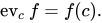
Let $P_{n}$ denote the vector space of real-valued polynomial functions of degree $\leq n$ defined on an interval $[a,b].$ If $c\in [a,b],$ then let $\operatorname {ev} _{c}:P_{n}\to \mathbb {R}$ be the evaluation functional $\operatorname {ev} _{c}f=f(c).$ The mapping $f\mapsto f(c)$ is linear since ${\begin{aligned}(f+g)(c)&=f(c)+g(c)\\(\alpha f)(c)&=\alpha f(c).\end{aligned}}$

If $x_{0},\ldots ,x_{n}$ are $n+1$ distinct points in $[a,b],$ then the evaluation functionals $\operatorname {ev} _{x_{i}},$ $i=0,\ldots ,n$ form a basis of the dual space of $P_{n}$ (Lax (1996) proves this last fact using Lagrange interpolation).

Non-example

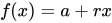
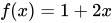
A function $f$ having the equation of a line $f(x)=a+rx$ with $a\neq 0$ (for example, $f(x)=1+2x$ ) is not a linear functional on $\mathbb {R}$ , since it is not linear. It is, however, affine-linear.

02Visualization

In finite dimensions, a linear functional can be visualized in terms of its level sets, the sets of vectors which map to a given value. In three dimensions, the level sets of a linear functional are a family of mutually parallel planes; in higher dimensions, they are parallel hyperplanes. This method of visualizing linear functionals is sometimes introduced in general relativity texts, such as Gravitation by Misner, Thorne & Wheeler (1973).

03Applications

Application to quadrature

If $x_{0},\ldots ,x_{n}$ are $n+1$ distinct points in [a, b], then the linear functionals $\operatorname {ev} _{x_{i}}:f\mapsto f\left(x_{i}\right)$ defined above form a basis of the dual space of P_n, the space of polynomials of degree $\leq n.$ The integration functional I is also a linear functional on P_n, and so can be expressed as a linear combination of these basis elements. In symbols, there are coefficients $a_{0},\ldots ,a_{n}$ for which $I(f)=a_{0}f(x_{0})+a_{1}f(x_{1})+\dots +a_{n}f(x_{n})$ for all $f\in P_{n}.$ This forms the foundation of the theory of numerical quadrature.

In quantum mechanics

Linear functionals are particularly important in quantum mechanics. Quantum mechanical systems are represented by Hilbert spaces, which are anti, isomorphic to their own dual spaces. A state of a quantum mechanical system can be identified with a linear functional. For more information see bra-ket notation.

Distributions

In the theory of generalized functions, certain kinds of generalized functions called distributions can be realized as linear functionals on spaces of test functions.

04Dual vectors and bilinear forms

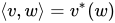
Every non-degenerate bilinear form on a finite-dimensional vector space $V$ induces an isomorphism $V\rightarrow V^{*}:v\mapsto v^{*}$ such that $v^{*}(w):=\langle v,w\rangle \quad \forall w\in V,$

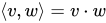
where the bilinear form on $V$ is denoted $\langle \,\cdot \,,\,\cdot \,\rangle$ (for instance, in Euclidean space, $\langle v,w\rangle =v\cdot w$ is the dot product of $v$ and $w$ ).

The inverse isomorphism is $V^{*}\rightarrow V:v^{*}\mapsto v$ , where $v$ is the unique element of $V$ such that $\langle v,w\rangle =v^{*}(w)$ for all $w\in V$ .

The above defined vector $v^{*}\in V^{*}$ is said to be the dual vector of $v\in V$ .

In an infinite dimensional Hilbert space, analogous results hold by the Riesz representation theorem. There is a mapping $V\mapsto V^{*}$ from $V$ into its continuous dual space $V^{*}$ .

05Relationship to bases

Basis of the dual space

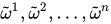
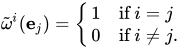
Let the vector space V have a basis $\mathbf {e} _{1},\mathbf {e} _{2},\dots ,\mathbf {e} _{n}$ , not necessarily orthogonal. Then the dual space $V^{*}$ has a basis ${\tilde {\omega }}^{1},{\tilde {\omega }}^{2},\dots ,{\tilde {\omega }}^{n}$ called the dual basis defined by the special property that ${\tilde {\omega }}^{i}(\mathbf {e} _{j})={\begin{cases}1&{\text{if}}\ i=j\\0&{\text{if}}\ i\neq j.\end{cases}}$

Or, more succinctly, ${\tilde {\omega }}^{i}(\mathbf {e} _{j})=\delta _{ij}$

where $\delta _{ij}$ is the Kronecker delta. Here the superscripts of the basis functionals are not exponents but are instead contravariant indices.

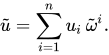
A linear functional ${\tilde {u}}$ belonging to the dual space ${\tilde {V}}$ can be expressed as a linear combination of basis functionals, with coefficients ("components") u_i, ${\tilde {u}}=\sum _{i=1}^{n}u_{i}\,{\tilde {\omega }}^{i}.$

Then, applying the functional ${\tilde {u}}$ to a basis vector $\mathbf {e} _{j}$ yields ${\tilde {u}}(\mathbf {e} _{j})=\sum _{i=1}^{n}\left(u_{i}\,{\tilde {\omega }}^{i}\right)\mathbf {e} _{j}=\sum _{i}u_{i}\left[{\tilde {\omega }}^{i}\left(\mathbf {e} _{j}\right)\right]$

due to linearity of scalar multiples of functionals and pointwise linearity of sums of functionals. Then ${\begin{aligned}{\tilde {u}}({\mathbf {e} }_{j})&=\sum _{i}u_{i}\left[{\tilde {\omega }}^{i}\left({\mathbf {e} }_{j}\right)\right]\\&=\sum _{i}u_{i}{\delta }_{ij}\\&=u_{j}.\end{aligned}}$

So each component of a linear functional can be extracted by applying the functional to the corresponding basis vector.

The dual basis and inner product

When the space V carries an inner product, then it is possible to write explicitly a formula for the dual basis of a given basis. Let V have (not necessarily orthogonal) basis $\mathbf {e} _{1},\dots ,\mathbf {e} _{n}.$ In three dimensions (n = 3), the dual basis can be written explicitly ${\tilde {\omega }}^{i}(\mathbf {v} )={\frac {1}{2}}\left\langle {\frac {\sum _{j=1}^{3}\sum _{k=1}^{3}\varepsilon ^{ijk}\,(\mathbf {e} _{j}\times \mathbf {e} _{k})}{\mathbf {e} _{1}\cdot \mathbf {e} _{2}\times \mathbf {e} _{3}}},\mathbf {v} \right\rangle ,$ for $i=1,2,3,$ where ε is the Levi-Civita symbol and $\langle \cdot ,\cdot \rangle$ the inner product (or dot product) on V.

In higher dimensions, this generalizes as follows ${\tilde {\omega }}^{i}(\mathbf {v} )=\left\langle {\frac {\sum _{1\leq i_{2}<i_{3}<\dots <i_{n}\leq n}\varepsilon ^{ii_{2}\dots i_{n}}(\star \mathbf {e} _{i_{2}}\wedge \cdots \wedge \mathbf {e} _{i_{n}})}{\star (\mathbf {e} _{1}\wedge \cdots \wedge \mathbf {e} _{n})}},\mathbf {v} \right\rangle ,$ where $\star$ is the Hodge star operator.

06Over a ring

Modules over a ring are generalizations of vector spaces, which removes the restriction that coefficients belong to a field. Given a module M over a ring R, a linear form on M is a linear map from M to R, where the latter is considered as a module over itself. The space of linear forms is always denoted Hom_k(V, k), whether k is a field or not. It is a right module if V is a left module.

The existence of "enough" linear forms on a module is equivalent to projectivity.

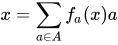
Dual Basis Lemma, An R-module M is projective if and only if there exists a subset $A\subset M$ and linear forms $\{f_{a}\mid a\in A\}$ such that, for every $x\in M,$ only finitely many $f_{a}(x)$ are nonzero, and $x=\sum _{a\in A}{f_{a}(x)a}$

07Change of field

Suppose that $X$ is a vector space over $\mathbb {C} .$ Restricting scalar multiplication to $\mathbb {R}$ gives rise to a real vector space $X_{\mathbb {R} }$ called the realification of $X.$ Any vector space $X$ over $\mathbb {C}$ is also a vector space over $\mathbb {R} ,$ endowed with a complex structure; that is, there exists a real vector subspace $X_{\mathbb {R} }$ such that we can (formally) write $X=X_{\mathbb {R} }\oplus X_{\mathbb {R} }i$ as $\mathbb {R}$ -vector spaces.

Real versus complex linear functionals

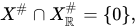
Every linear functional on $X$ is complex-valued while every linear functional on $X_{\mathbb {R} }$ is real-valued. If $\dim X\neq 0$ then a linear functional on either one of $X$ or $X_{\mathbb {R} }$ is non-trivial (meaning not identically $0$ ) if and only if it is surjective (because if $\varphi (x)\neq 0$ then for any scalar $s,$ $\varphi \left((s/\varphi (x))x\right)=s$ ), where the image of a linear functional on $X$ is $\mathbb {C}$ while the image of a linear functional on $X_{\mathbb {R} }$ is $\mathbb {R} .$ Consequently, the only function on $X$ that is both a linear functional on $X$ and a linear function on $X_{\mathbb {R} }$ is the trivial functional; in other words, $X^{\#}\cap X_{\mathbb {R} }^{\#}=\{0\},$ where $\,{\cdot }^{\#}$ denotes the space's algebraic dual space. However, every $\mathbb {C}$ -linear functional on $X$ is an $\mathbb {R}$ -linear operator (meaning that it is additive and homogeneous over $\mathbb {R}$ ), but unless it is identically $0,$ it is not an $\mathbb {R}$ -linear functional on $X$ because its range (which is $\mathbb {C}$ ) is 2-dimensional over $\mathbb {R} .$ Conversely, a non-zero $\mathbb {R}$ -linear functional has range too small to be a $\mathbb {C}$ -linear functional as well.

Real and imaginary parts

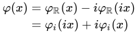
If $\varphi \in X^{\#}$ then denote its real part by $\varphi _{\mathbb {R} }:=\operatorname {Re} \varphi$ and its imaginary part by $\varphi _{i}:=\operatorname {Im} \varphi .$ Then $\varphi _{\mathbb {R} }:X\to \mathbb {R}$ and $\varphi _{i}:X\to \mathbb {R}$ are linear functionals on $X_{\mathbb {R} }$ and $\varphi =\varphi _{\mathbb {R} }+i\varphi _{i}.$ The fact that $z=\operatorname {Re} z-i\operatorname {Re} (iz)=\operatorname {Im} (iz)+i\operatorname {Im} z$ for all $z\in \mathbb {C}$ implies that for all $x\in X,$ ${\begin{alignedat}{4}\varphi (x)&=\varphi _{\mathbb {R} }(x)-i\varphi _{\mathbb {R} }(ix)\\&=\varphi _{i}(ix)+i\varphi _{i}(x)\\\end{alignedat}}$ and consequently, that $\varphi _{i}(x)=-\varphi _{\mathbb {R} }(ix)$ and $\varphi _{\mathbb {R} }(x)=\varphi _{i}(ix).$

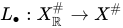
The assignment $\varphi \mapsto \varphi _{\mathbb {R} }$ defines a bijective $\mathbb {R}$ -linear operator $X^{\#}\to X_{\mathbb {R} }^{\#}$ whose inverse is the map $L_{\bullet }:X_{\mathbb {R} }^{\#}\to X^{\#}$ defined by the assignment $g\mapsto L_{g}$ that sends $g:X_{\mathbb {R} }\to \mathbb {R}$ to the linear functional $L_{g}:X\to \mathbb {C}$ defined by $L_{g}(x):=g(x)-ig(ix)\quad {\text{ for all }}x\in X.$ The real part of $L_{g}$ is $g$ and the bijection $L_{\bullet }:X_{\mathbb {R} }^{\#}\to X^{\#}$ is an $\mathbb {R}$ -linear operator, meaning that $L_{g+h}=L_{g}+L_{h}$ and $L_{rg}=rL_{g}$ for all $r\in \mathbb {R}$ and $g,h\in X_{\mathbb {R} }^{\#}.$ Similarly for the imaginary part, the assignment $\varphi \mapsto \varphi _{i}$ induces an $\mathbb {R}$ -linear bijection $X^{\#}\to X_{\mathbb {R} }^{\#}$ whose inverse is the map $X_{\mathbb {R} }^{\#}\to X^{\#}$ defined by sending $I\in X_{\mathbb {R} }^{\#}$ to the linear functional on $X$ defined by $x\mapsto I(ix)+iI(x).$

This relationship was discovered by Henry Löwig in 1934 (although it is usually credited to F. Murray), and can be generalized to arbitrary finite extensions of a field in the natural way. It has many important consequences, some of which will now be described.

Properties and relationships

Suppose $\varphi :X\to \mathbb {C}$ is a linear functional on $X$ with real part $\varphi _{\mathbb {R} }:=\operatorname {Re} \varphi$ and imaginary part $\varphi _{i}:=\operatorname {Im} \varphi .$

Then $\varphi =0$ if and only if $\varphi _{\mathbb {R} }=0$ if and only if $\varphi _{i}=0.$

Assume that $X$ is a topological vector space. Then $\varphi$ is continuous if and only if its real part $\varphi _{\mathbb {R} }$ is continuous, if and only if $\varphi$ 's imaginary part $\varphi _{i}$ is continuous. That is, either all three of $\varphi ,\varphi _{\mathbb {R} },$ and $\varphi _{i}$ are continuous or none are continuous. This remains true if the word "continuous" is replaced with the word "bounded". In particular, $\varphi \in X^{\prime }$ if and only if $\varphi _{\mathbb {R} }\in X_{\mathbb {R} }^{\prime }$ where the prime denotes the space's continuous dual space.

Let $B\subseteq X.$ If $uB\subseteq B$ for all scalars $u\in \mathbb {C}$ of unit length (meaning $|u|=1$ ) then $\sup _{b\in B}|\varphi (b)|=\sup _{b\in B}\left|\varphi _{\mathbb {R} }(b)\right|.$ Similarly, if $\varphi _{i}:=\operatorname {Im} \varphi :X\to \mathbb {R}$ denotes the complex part of $\varphi$ then $iB\subseteq B$ implies $\sup _{b\in B}\left|\varphi _{\mathbb {R} }(b)\right|=\sup _{b\in B}\left|\varphi _{i}(b)\right|.$ If $X$ is a normed space with norm $\|\cdot \|$ and if $B=\{x\in X:\|x\|\leq 1\}$ is the closed unit ball then the supremums above are the operator norms (defined in the usual way) of $\varphi ,\varphi _{\mathbb {R} },$ and $\varphi _{i}$ so that $\|\varphi \|=\left\|\varphi _{\mathbb {R} }\right\|=\left\|\varphi _{i}\right\|.$ This conclusion extends to the analogous statement for polars of balanced sets in general topological vector spaces.

If $X$ is a complex Hilbert space with a (complex) inner product $\langle \,\cdot \,|\,\cdot \,\rangle$ that is antilinear in its first coordinate (and linear in the second) then $X_{\mathbb {R} }$ becomes a real Hilbert space when endowed with the real part of $\langle \,\cdot \,|\,\cdot \,\rangle .$ Explicitly, this real inner product on $X_{\mathbb {R} }$ is defined by $\langle x|y\rangle _{\mathbb {R} }:=\operatorname {Re} \langle x|y\rangle$ for all $x,y\in X$ and it induces the same norm on $X$ as $\langle \,\cdot \,|\,\cdot \,\rangle$ because ${\sqrt {\langle x|x\rangle _{\mathbb {R} }}}={\sqrt {\langle x|x\rangle }}$ for all vectors $x.$ Applying the Riesz representation theorem to $\varphi \in X^{\prime }$ (resp. to $\varphi _{\mathbb {R} }\in X_{\mathbb {R} }^{\prime }$ ) guarantees the existence of a unique vector $f_{\varphi }\in X$ (resp. $f_{\varphi _{\mathbb {R} }}\in X_{\mathbb {R} }$ ) such that $\varphi (x)=\left\langle f_{\varphi }|\,x\right\rangle$ (resp. $\varphi _{\mathbb {R} }(x)=\left\langle f_{\varphi _{\mathbb {R} }}|\,x\right\rangle _{\mathbb {R} }$ ) for all vectors $x.$ The theorem also guarantees that $\left\|f_{\varphi }\right\|=\|\varphi \|_{X^{\prime }}$ and $\left\|f_{\varphi _{\mathbb {R} }}\right\|=\left\|\varphi _{\mathbb {R} }\right\|_{X_{\mathbb {R} }^{\prime }}.$ It is readily verified that $f_{\varphi }=f_{\varphi _{\mathbb {R} }}.$ Now $\left\|f_{\varphi }\right\|=\left\|f_{\varphi _{\mathbb {R} }}\right\|$ and the previous equalities imply that $\|\varphi \|_{X^{\prime }}=\left\|\varphi _{\mathbb {R} }\right\|_{X_{\mathbb {R} }^{\prime }},$ which is the same conclusion that was reached above.

08In infinite dimensions

Below, all vector spaces are over either the real numbers $\mathbb {R}$ or the complex numbers $\mathbb {C} .$

If $V$ is a topological vector space, the space of continuous linear functionals, the continuous dual, is often simply called the dual space. If $V$ is a Banach space, then so is its (continuous) dual. To distinguish the ordinary dual space from the continuous dual space, the former is sometimes called the algebraic dual space. In finite dimensions, every linear functional is continuous, so the continuous dual is the same as the algebraic dual, but in infinite dimensions the continuous dual is a proper subspace of the algebraic dual.

A linear functional f on a (not necessarily locally convex) topological vector space X is continuous if and only if there exists a continuous seminorm p on X such that $|f|\leq p.$

Characterizing closed subspaces

Continuous linear functionals have nice properties for analysis: a linear functional is continuous if and only if its kernel is closed, and a non-trivial continuous linear functional is an open map, even if the (topological) vector space is not complete.

Hyperplanes and maximal subspaces

A vector subspace $M$ of $X$ is called maximal if $M\subsetneq X$ (meaning $M\subseteq X$ and $M\neq X$ ) and does not exist a vector subspace $N$ of $X$ such that $M\subsetneq N\subsetneq X.$ A vector subspace $M$ of $X$ is maximal if and only if it is the kernel of some non-trivial linear functional on $X$ (that is, $M=\ker f$ for some linear functional $f$ on $X$ that is not identically 0). An affine hyperplane in $X$ is a translate of a maximal vector subspace. By linearity, a subset $H$ of $X$ is a affine hyperplane if and only if there exists some non-trivial linear functional $f$ on $X$ such that $H=f^{-1}(1)=\{x\in X:f(x)=1\}.$ If $f$ is a linear functional and $s\neq 0$ is a scalar then $f^{-1}(s)=s\left(f^{-1}(1)\right)=\left({\frac {1}{s}}f\right)^{-1}(1).$ This equality can be used to relate different level sets of $f.$ Moreover, if $f\neq 0$ then the kernel of $f$ can be reconstructed from the affine hyperplane $H:=f^{-1}(1)$ by $\ker f=H-H.$

Relationships between multiple linear functionals

Any two linear functionals with the same kernel are proportional (i.e. scalar multiples of each other). This fact can be generalized to the following theorem.

Theorem, If $f,g_{1},\ldots ,g_{n}$ are linear functionals on X, then the following are equivalent:

f can be written as a linear combination of $g_{1},\ldots ,g_{n}$ ; that is, there exist scalars $s_{1},\ldots ,s_{n}$ such that $sf=s_{1}g_{1}+\cdots +s_{n}g_{n}$ ;
$\bigcap _{i=1}^{n}\ker g_{i}\subseteq \ker f$ ;
there exists a real number r such that $|f(x)|\leq r\max _{i}|g_{i}(x)|$ for all $x\in X$ .

If f is a non-trivial linear functional on X with kernel N, $x\in X$ satisfies $f(x)=1,$ and U is a balanced subset of X, then $N\cap (x+U)=\varnothing$ if and only if $|f(u)|<1$ for all $u\in U.$

Hahn-Banach theorem

Any (algebraic) linear functional on a vector subspace can be extended to the whole space; for example, the evaluation functionals described above can be extended to the vector space of polynomials on all of $\mathbb {R} .$ However, this extension cannot always be done while keeping the linear functional continuous. The Hahn-Banach family of theorems gives conditions under which this extension can be done. For example,

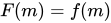
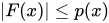
Hahn-Banach dominated extension theorem (Rudin 1991, Th. 3.2), If $p:X\to \mathbb {R}$ is a sublinear function, and $f:M\to \mathbb {R}$ is a linear functional on a linear subspace $M\subseteq X$ which is dominated by p on M, then there exists a linear extension $F:X\to \mathbb {R}$ of f to the whole space X that is dominated by p, i.e., there exists a linear functional F such that $F(m)=f(m)$ for all $m\in M,$ and $|F(x)|\leq p(x)$ for all $x\in X.$

Equicontinuity of families of linear functionals

Let X be a topological vector space (TVS) with continuous dual space $X'.$

For any subset H of $X',$ the following are equivalent:

H is equicontinuous;
H is contained in the polar of some neighborhood of $0$ in X;
the (pre)polar of H is a neighborhood of $0$ in X;

If H is an equicontinuous subset of $X'$ then the following sets are also equicontinuous: the weak-* closure, the balanced hull, the convex hull, and the convex balanced hull. Moreover, Alaoglu's theorem implies that the weak-* closure of an equicontinuous subset of $X'$ is weak-* compact (and thus that every equicontinuous subset weak-* relatively compact).

Watch videos about Linear formExplainers and documentaries on YouTube (opens in a new tab)

Sources and credits

This article is adapted from the Wikipedia article “Linear form”, written by its contributors and licensed under CC BY-SA 4.0. Fathomly has changed the layout, removed citation markers, navigation and maintenance notices, and adjusted punctuation. This adapted version is shared under the same license. For references, see the original article.

Images, from Wikimedia Commons:

Gradient 1-form.svg by Maschen, CC0
1-form linear functional.svg by Maschen, CC0

Fathomly is not affiliated with or endorsed by the Wikimedia Foundation. Spotted a problem? Tell us.

Linear form

01Examples

Linear functionals in Rⁿ

Trace of a square matrix

(Definite) integration

Evaluation

Non-example

02Visualization

03Applications

Application to quadrature

In quantum mechanics

Distributions

04Dual vectors and bilinear forms

05Relationship to bases

Basis of the dual space

The dual basis and inner product

06Over a ring

07Change of field

Real versus complex linear functionals

Real and imaginary parts

Properties and relationships

08In infinite dimensions

Characterizing closed subspaces

Hyperplanes and maximal subspaces

Relationships between multiple linear functionals

Hahn-Banach theorem

Equicontinuity of families of linear functionals

Sources and credits

Related topics

Discontinuous linear map

Locally convex topological vector space

Positive linear functional

Linear form

01Examples

Linear functionals in Rn

Trace of a square matrix

(Definite) integration

Evaluation

Non-example

02Visualization

03Applications

Application to quadrature

In quantum mechanics

Distributions

04Dual vectors and bilinear forms

05Relationship to bases

Basis of the dual space

The dual basis and inner product

06Over a ring

07Change of field

Real versus complex linear functionals

Real and imaginary parts

Properties and relationships

08In infinite dimensions

Characterizing closed subspaces

Hyperplanes and maximal subspaces

Relationships between multiple linear functionals

Hahn-Banach theorem

Equicontinuity of families of linear functionals

Sources and credits

Related topics

Discontinuous linear map

Locally convex topological vector space

Positive linear functional

Linear functionals in Rⁿ