Encyclopedia

Limit (mathematics)

Value approached by a mathematical object

Wikipedia contributorsAdapted for Fathomly · View authors

16 min read
Source updated September 15, 2026

In mathematics, a limit is the value that a function (or sequence) approaches as the argument (or index) approaches some value. Limits of functions are essential to calculus and mathematical analysis, and are used to define continuity, derivatives, and integrals. The concept of a limit of a sequence is further generalized to the concept of a limit of a topological net, and is closely related to limit and direct limit in category theory. The limit inferior and limit superior provide generalizations of the concept of a limit which are particularly relevant when the limit at a point may not exist.

01Notation

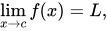
In formulas, a limit of a function is usually written as $\lim _{x\to c}f(x)=L,$ and is read as "the limit of $f$ of $x$ as $x$ approaches $c$ equals $L$ ". This means that the value of the function $f$ can be made arbitrarily close to $L$ , by choosing $x$ sufficiently close to $c$ . Alternatively, the fact that a function $f$ approaches the limit $L$ as $x$ approaches $c$ is sometimes denoted by a right arrow (→ or $\rightarrow$ ), as in $f(x)\to L{\text{ as }}x\to c,$ or in

$f(x){\xrightarrow[{x\to c}]{}}L,$

which reads " $f$ of $x$ tends to $L$ as $x$ tends to $c$ ".

A function f(x) for which the limit at infinity is L. For any arbitrary distance ε, there must be a value S such that the function stays within L ± ε for all ''S''"}},"i":0}}]}' id="mwAQk">x > S.

02History

According to Hankel (1871), the modern concept of limit originates from Proposition X.1 of Euclid's Elements, which forms the basis of the Method of exhaustion found in Euclid and Archimedes: "Two unequal magnitudes being set out, if from the greater there is subtracted a magnitude greater than its half, and from that which is left a magnitude greater than its half, and if this process is repeated continually, then there will be left some magnitude less than the lesser magnitude set out."

Grégoire de Saint-Vincent gave the first definition of limit (terminus) of a geometric series in his work Opus Geometricum (1647): "The terminus of a progression is the end of the series, which none progression can reach, even not if she is continued in infinity, but which she can approach nearer than a given segment."

In the Scholium to Principia in 1687, Isaac Newton had a clear definition of a limit, stating that "Those ultimate ratios ... are not actually ratios of ultimate quantities, but limits ... which they can approach so closely that their difference is less than any given quantity". Bruce Pourciau further argues that, in addition to Newton actually having a more sophisticated understanding of limits than he is generally credited with, he also provided the first epsilon argument.

The modern definition of a limit goes back to Bernard Bolzano who, in 1817, developed the basics of the epsilon-delta technique to define continuous functions. However, his work remained unknown to other mathematicians until thirty years after his death.

Augustin-Louis Cauchy in 1821, followed by Karl Weierstrass, formalized the definition of the limit of a function which became known as the (ε, δ)-definition of limit.

The modern notation of placing the arrow below the limit symbol was invented by John Gaston Leathem in 1905 and popularized by G. H. Hardy's 1908 textbook A Course of Pure Mathematics.

03Types of limits

In sequences

Real numbers

A sequence of real numbers $a_{0},a_{1},\dots$ is said to converge to a limit $L$ if the terms of the sequence give an arbitrarily good approximation of the number $L$ , after discarding finitely many initial terms. An example is the sequence $0,0.3,0.33,0.333,0.3333,$ and so on. Each term in the sequence is an approximation to the rational number $1/3=0.333\ldots$ . If an approximation is desired that lies within a given error $\epsilon$ , then all of the terms of the sequence except finitely many lie within the target error. For example, to get within $\epsilon =0.001$ of $1/3$ , the approximations $0$ , $0.3$ , and $0.33$ are outside the error window, but after discarding those three approximations, all of the remaining approximations are within the error range $\epsilon =0.001$ . The same approximation property holds for every positive error $\epsilon$ .

More precisely, a sequence $\{a_{n}\}_{n\in \mathbb {N} }$ of real numbers is said to be convergent if there exists an $L\in \mathbb {R}$ such that for each positive real number $\epsilon$ , there exists a positive integer $N$ (depending on $\epsilon$ ) such that every term $a_{n}$ with $n>N$ is within distance $\epsilon$ of $L$ . The number $L$ is unique, when it exists. It is called the limit of the sequence $\{a_{n}\}_{n\in \mathbb {N} }$ , and this is written $\lim _{n\to \infty }a_{n}=L.$

The definition of the limit of a sequence can thus be summarized:

$\lim _{n\to \infty }a_{n}=L$ means that for every $\epsilon >0$ , there exists $N\in \mathbb {N}$ such that $|a_{n}-L|<\epsilon$ for all $n>N$ .

If such an $L$ does not exist, $\{a_{n}\}_{n\in \mathbb {N} }$ is said to be divergent.

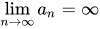
A sequence is said to tend to infinity if all but finitely many terms exceed each given number. An example is the sequence $1,2,3,\ldots$ of positive integers. This tends to infinity because, for any given bound $M$ , every element of the sequence is greater than $M$ after discarding the finite number that are not. Formally, $\{a_{n}\}_{n\in \mathbb {N} }$ tends to infinity if, given any real $M$ , there exists a positive integer $N$ such that $a_{n}>M$ for every $n>N$ . This is written as $\lim _{n\to \infty }a_{n}=\infty$ .

Similarly, the sequence is said to tend to negative infinity if all but finitely many terms are less than any given lower bound. This is written as $\lim _{n\to \infty }a_{n}=-\infty$ .

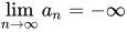
In each case where $\lim _{n\to \infty }a_{n}=\infty$ or $\lim _{n\to \infty }a_{n}=-\infty$ , the sequence is said to have an infinite limit. But it does not have a limit in the sense of being convergent to a real number, since $\infty$ and $-\infty$ are not real numbers.

Metric space

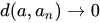
The discussion of sequences above is for sequences of real numbers. The notion of limits can be defined for sequences valued in more abstract spaces, such as metric spaces. If $M$ is a metric space with distance function $d$ , and $\{a_{n}\}_{n\geq 0}$ is a sequence in $M$ , then the limit (when it exists) of the sequence is an element $a\in M$ such that, given $\varepsilon >0$ , there exists an $N$ such that for each $n>N$ , we have $d(a,a_{n})<\varepsilon .$ An equivalent statement is that $a_{n}\rightarrow a$ if the sequence of real numbers $d(a,a_{n})\rightarrow 0$ .

Example: ℝⁿ

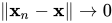
An important example is the space of $n$ -dimensional real vectors, with elements $\mathbf {x} =(x_{1},\cdots ,x_{n})$ where each of the $x_{i}$ are real, an example of a suitable distance function is the Euclidean distance, defined by $d(\mathbf {x} ,\mathbf {y} )=\|\mathbf {x} -\mathbf {y} \|={\sqrt {\sum _{i}(x_{i}-y_{i})^{2}}}.$ The sequence of points $\{\mathbf {x} _{n}\}_{n\geq 0}$ converges to $\mathbf {x}$ if the limit exists and $\|\mathbf {x} _{n}-\mathbf {x} \|\rightarrow 0$ .

Topological space

In some sense the most abstract space in which limits can be defined are topological spaces. If $X$ is a topological space with topology $\tau$ , and $\{a_{n}\}_{n\geq 0}$ is a sequence in $X$ , then the limit (when it exists) of the sequence is a point $a\in X$ such that, given a (open) neighborhood $U\in \tau$ of $a$ , there exists an $N$ such that for every $n>N$ , $a_{n}\in U$ is satisfied. In this case, the limit (if it exists) may not be unique. However it must be unique if $X$ is a Hausdorff space.

Function space

This section deals with the idea of limits of sequences of functions, not to be confused with the idea of limits of functions, discussed below.

The field of functional analysis partly seeks to identify useful notions of convergence on function spaces. For example, consider the space of functions from a generic set $E$ to $\mathbb {R}$ . Given a sequence of functions $\{f_{n}\}_{n>0}$ such that each is a function $f_{n}:E\rightarrow \mathbb {R}$ , suppose that there exists a function such that for each $x\in E$ , $f_{n}(x)\rightarrow f(x){\text{ or equivalently }}\lim _{n\rightarrow \infty }f_{n}(x)=f(x).$

Then the sequence $f_{n}$ is said to converge pointwise to $f$ . However, such sequences can exhibit unexpected behavior. For example, it is possible to construct a sequence of continuous functions which has a discontinuous pointwise limit.

Another notion of convergence is uniform convergence. The uniform distance between two functions $f,g:E\rightarrow \mathbb {R}$ is the maximum difference between the two functions as the argument $x\in E$ is varied. That is, $d(f,g)=\max _{x\in E}|f(x)-g(x)|.$ Then the sequence $f_{n}$ is said to uniformly converge or have a uniform limit of $f$ if $f_{n}\rightarrow f$ with respect to this distance. The uniform limit has "nicer" properties than the pointwise limit. For example, the uniform limit of a sequence of continuous functions is continuous.

Many different notions of convergence can be defined on function spaces. This is sometimes dependent on the regularity of the space. Prominent examples of function spaces with some notion of convergence are Lp spaces and Sobolev space.

In functions

Suppose f is a real-valued function and c is a real number. Intuitively speaking, the expression

$\lim _{x\to c}f(x)=L$

means that f(x) can be made to be as close to L as desired, by making x sufficiently close to c. In that case, the above equation can be read as "the limit of f of x, as x approaches c, is L".

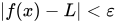
Formally, the definition of the "limit of $f(x)$ as $x$ approaches $c$ " is given as follows. The limit is a real number $L$ so that, given an arbitrary real number $\varepsilon >0$ (thought of as the "error"), there is a $\delta >0$ such that, for any $x$ satisfying $0<|x-c|<\delta$ , it holds that $|f(x)-L|<\varepsilon$ . This is known as the (ε, δ)-definition of limit.

The inequality $0<|x-c|$ is used to exclude $c$ from the set of points under consideration, but some authors do not include this in their definition of limits, replacing $0<|x-c|<\delta$ with simply $|x-c|<\delta$ . This replacement is equivalent to additionally requiring that $f$ be continuous at $c$ .

It can be proven that there is an equivalent definition which makes manifest the connection between limits of sequences and limits of functions. The equivalent definition is given as follows. First observe that for every sequence $\{x_{n}\}$ in the domain of $f$ , there is an associated sequence $\{f(x_{n})\}$ , the image of the sequence under $f$ . The limit is a real number $L$ so that, for all sequences $x_{n}\rightarrow c$ , the associated sequence $f(x_{n})\rightarrow L$ .

One-sided limit

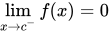
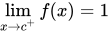
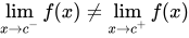
It is possible to define the notion of having a "left-handed" limit ("from below"), and a notion of a "right-handed" limit ("from above"). These need not agree. An example is given by the positive indicator function, $f:\mathbb {R} \rightarrow \mathbb {R}$ , defined such that $f(x)=0$ if $x\leq 0$ , and $f(x)=1$ if $x>0$ . At $x=0$ , the function has a "left-handed limit" of 0, a "right-handed limit" of 1, and its limit does not exist. Symbolically, this can be stated as, for this example, $\lim _{x\to c^{-}}f(x)=0$ , and $\lim _{x\to c^{+}}f(x)=1$ , and from this it can be deduced $\lim _{x\to c}f(x)$ does not exist, because $\lim _{x\to c^{-}}f(x)\neq \lim _{x\to c^{+}}f(x)$ .

Infinity in limits of functions

It is possible to define the notion of "tending to infinity" in the domain of $f$ , $\lim _{x\rightarrow +\infty }f(x)=L.$

This could be considered equivalent to the limit as a reciprocal tends to 0: $\lim _{x'\rightarrow 0^{+}}f(1/x')=L.$

or it can be defined directly: the "limit of $f$ as $x$ tends to positive infinity" is defined as a value $L$ such that, given any real $\varepsilon >0$ , there exists an $M>0$ so that for all $x>M$ , $|f(x)-L|<\varepsilon$ . The definition for sequences is equivalent: As $n\rightarrow +\infty$ , we have $f(x_{n})\rightarrow L$ .

In these expressions, the infinity is normally considered to be signed ( $+\infty$ or $-\infty$ ) and corresponds to a one-sided limit of the reciprocal. A two-sided infinite limit can be defined, but an author would explicitly write $\pm \infty$ to be clear.

It is also possible to define the notion of "tending to infinity" in the value of $f$ , $\lim _{x\rightarrow c}f(x)=\infty .$

Again, this could be defined in terms of a reciprocal: $\lim _{x\rightarrow c}{\frac {1}{f(x)}}=0.$

Or a direct definition can be given as follows: given any real number $M>0$ , there is a $\delta >0$ so that for $0<|x-c|<\delta$ , the absolute value of the function $|f(x)|>M$ . A sequence can also have an infinite limit: as $n\rightarrow \infty$ , the sequence $f(x_{n})\rightarrow \infty$ .

This direct definition is easier to extend to one-sided infinite limits. While mathematicians do talk about functions approaching limits "from above" or "from below", there is not a standard mathematical notation for this as there is for one-sided limits.

Nonstandard analysis

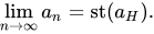
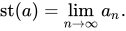
In non-standard analysis (which involves a hyperreal enlargement of the number system), the limit of a sequence $(a_{n})$ can be expressed as the standard part of the value $a_{H}$ of the natural extension of the sequence at an infinite hypernatural index n = H. Thus, $\lim _{n\to \infty }a_{n}=\operatorname {st} (a_{H}).$ Here, the standard part function "st" rounds off each finite hyperreal number to the nearest real number (the difference between them is infinitesimal). This formalizes the natural intuition that for "very large" values of the index, the terms in the sequence are "very close" to the limit value of the sequence. Conversely, the standard part of a hyperreal $a=[a_{n}]$ represented in the ultrapower construction by a Cauchy sequence $(a_{n})$ , is simply the limit of that sequence: $\operatorname {st} (a)=\lim _{n\to \infty }a_{n}.$ In this sense, taking the limit and taking the standard part are equivalent procedures.

Limit sets

Limit set of a sequence

Let $\{a_{n}\}_{n>0}$ be a sequence in a topological space $X$ . For concreteness, $X$ can be thought of as $\mathbb {R}$ , but the definitions hold more generally. The limit set is the set of points such that if there is a convergent subsequence $\{a_{n_{k}}\}_{k>0}$ with $a_{n_{k}}\rightarrow a$ , then $a$ belongs to the limit set. In this context, such an $a$ is sometimes called a limit point.

A use of this notion is to characterize the "long-term behavior" of oscillatory sequences. For example, consider the sequence $a_{n}=(-1)^{n}$ . Starting from n=1, the first few terms of this sequence are $-1,+1,-1,+1,\cdots$ . It can be checked that it is oscillatory, so has no limit, but has limit points $\{-1,+1\}$ .

Limit set of a trajectory

This notion is used in dynamical systems, to study limits of trajectories. Defining a trajectory to be a function $\gamma :\mathbb {R} \rightarrow X$ , the point $\gamma (t)$ is thought of as the "position" of the trajectory at "time" $t$ . The limit set of a trajectory is defined as follows. To any sequence of increasing times $\{t_{n}\}$ , there is an associated sequence of positions $\{x_{n}\}=\{\gamma (t_{n})\}$ . If $x$ is the limit set of the sequence $\{x_{n}\}$ for any sequence of increasing times, then $x$ is a limit set of the trajectory.

Technically, this is the $\omega$ -limit set. The corresponding limit set for sequences of decreasing time is called the $\alpha$ -limit set.

An illustrative example is the circle trajectory: $\gamma (t)=(\cos(t),\sin(t))$ . This has no unique limit, but for each $\theta \in \mathbb {R}$ , the point $(\cos(\theta ),\sin(\theta ))$ is a limit point, given by the sequence of times $t_{n}=\theta +2\pi n$ . But the limit points need not be attained on the trajectory. The trajectory $\gamma (t)=t/(1+t)(\cos(t),\sin(t))$ also has the unit circle as its limit set.

04Uses

Limits are used to define a number of important concepts in analysis.

Series

A particular expression of interest which is formalized as the limit of a sequence is sums of infinite series. These are "infinite sums" of real numbers, generally written as $\sum _{n=1}^{\infty }a_{n}.$ This is defined through limits as follows: given a sequence of real numbers $\{a_{n}\}$ , the sequence of partial sums is defined by $s_{n}=\sum _{i=1}^{n}a_{i}.$ If the limit of the sequence $\{s_{n}\}$ exists, the value of the expression $\sum _{n=1}^{\infty }a_{n}$ is defined to be the limit. Otherwise, the series is said to be divergent.

A classic example is the Basel problem, where $a_{n}=1/n^{2}$ . Then $\sum _{n=1}^{\infty }{\frac {1}{n^{2}}}={\frac {\pi ^{2}}{6}}.$

However, while for sequences there is essentially a unique notion of convergence, for series there are different notions of convergence. This is due to the fact that the expression $\sum _{n=1}^{\infty }a_{n}$ does not discriminate between different orderings of the sequence $\{a_{n}\}$ , while the convergence properties of the sequence of partial sums can depend on the ordering of the sequence.

A series which converges for all orderings is called unconditionally convergent. It can be proven to be equivalent to absolute convergence. This is defined as follows. A series is absolutely convergent if $\sum _{n=1}^{\infty }|a_{n}|$ is well defined. Furthermore, all possible orderings give the same value.

Otherwise, the series is conditionally convergent. A surprising result for conditionally convergent series is the Riemann series theorem: depending on the ordering, the partial sums can be made to converge to any real number, as well as $\pm \infty$ .

Power series

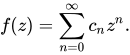
A useful application of the theory of sums of series is for power series. These are sums of series of the form $f(z)=\sum _{n=0}^{\infty }c_{n}z^{n}.$ Often $z$ is thought of as a complex number, and a suitable notion of convergence of complex sequences is needed. The set of values of $z\in \mathbb {C}$ for which the series sum converges is a circle, with its radius known as the radius of convergence.

Continuity of a function at a point

The definition of continuity at a point is given through limits.

The above definition of a limit is true even if $f(c)\neq L$ . Indeed, the function f need not even be defined at c. However, if $f(c)$ is defined and is equal to $L$ , then the function is said to be continuous at the point $c$ .

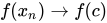
Equivalently, the function is continuous at $c$ if $f(x)\rightarrow f(c)$ as $x\rightarrow c$ , or in terms of sequences, whenever $x_{n}\rightarrow c$ , then $f(x_{n})\rightarrow f(c)$ .

An example of a limit where $f$ is not defined at $c$ is given below.

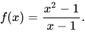
Consider the function

$f(x)={\frac {x^{2}-1}{x-1}}.$

then f(1) is not defined (see Indeterminate form), yet as x moves arbitrarily close to 1, f(x) correspondingly approaches 2:

f(0.9)	f(0.99)	f(0.999)	f(1.0)	f(1.001)	f(1.01)	f(1.1)
1.900	1.990	1.999	undefined	2.001	2.010	2.100

Thus, f(x) can be made arbitrarily close to the limit of 2, just by making x sufficiently close to 1. In other words, $\lim _{x\to 1}{\frac {x^{2}-1}{x-1}}=2.$

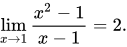
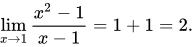
This can also be calculated algebraically, as ${\textstyle {\frac {x^{2}-1}{x-1}}={\frac {(x+1)(x-1)}{x-1}}=x+1$ for all real numbers x ≠ 1.

Now, since x + 1 is continuous in x at 1, we can now plug in 1 for x, leading to the equation $\lim _{x\to 1}{\frac {x^{2}-1}{x-1}}=1+1=2.$

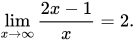
In addition to limits at finite values, functions can also have limits at infinity. For example, consider the function $f(x)={\frac {2x-1}{x}}$ where:

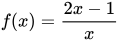
f(100) = 1.9900
f(1000) = 1.9990
f(10000) = 1.9999

As x becomes extremely large, the value of f(x) approaches 2, and the value of f(x) can be made as close to 2 as one could wish, by making x sufficiently large. So in this case, the limit of f(x) as x approaches infinity is 2, or in mathematical notation, $\lim _{x\to \infty }{\frac {2x-1}{x}}=2.$

Continuous functions

An important class of functions when considering limits are continuous functions. These are precisely those functions which preserve limits, in the sense that if $f$ is a continuous function, then whenever $a_{n}\rightarrow a$ in the domain of $f$ , then the limit $f(a_{n})$ exists and furthermore is $f(a)$ .

In the most general setting of topological spaces, a short proof is given below:

Let $f:X\rightarrow Y$ be a continuous function between topological spaces $X$ and $Y$ . By definition, for each open set $V$ in $Y$ , the preimage $f^{-1}(V)$ is open in $X$ .

Now suppose $a_{n}\rightarrow a$ is a sequence with limit $a$ in $X$ . Then $f(a_{n})$ is a sequence in $Y$ , and $f(a)$ is some point.

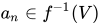
Choose a neighborhood $V$ of $f(a)$ . Then $f^{-1}(V)$ is an open set (by continuity of $f$ ) which in particular contains $a$ , and therefore $f^{-1}(V)$ is a neighborhood of $a$ . By the convergence of $a_{n}$ to $a$ , there exists an $N$ such that for $n>N$ , we have $a_{n}\in f^{-1}(V)$ .

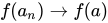
Then applying $f$ to both sides gives that, for the same $N$ , for each $n>N$ we have $f(a_{n})\in V$ . Originally $V$ was an arbitrary neighborhood of $f(a)$ , so $f(a_{n})\rightarrow f(a)$ . This concludes the proof.

In real analysis, for the more concrete case of real-valued functions defined on a subset $E\subset \mathbb {R}$ , that is, $f:E\rightarrow \mathbb {R}$ , a continuous function may also be defined as a function which is continuous at every point of its domain.

Limit points

In topology, limits are used to define limit points of a subset of a topological space, which in turn give a useful characterization of closed sets.

In a topological space $X$ , consider a subset $S$ . A point $a$ is called a limit point if there is a sequence $\{a_{n}\}$ in $S\setminus \{a\}$ such that $a_{n}\rightarrow a$ .

The reason why $\{a_{n}\}$ is defined to be in $S\setminus \{a\}$ rather than just $S$ is illustrated by the following example. Take $X=\mathbb {R}$ and $S=[0,1]\cup \{2\}$ . Then $2\in S$ , and therefore is the limit of the constant sequence $2,2,\cdots$ . But $2$ is not a limit point of $S$ .

A closed set, which is defined to be the complement of an open set, is equivalently any set $C$ which contains all its limit points.

Derivative

The derivative is defined formally as a limit. In the scope of real analysis, the derivative is first defined for real functions $f$ defined on a subset $E\subset \mathbb {R}$ . The derivative at $x\in E$ is defined as follows. If the limit of ${\frac {f(x+h)-f(x)}{h}}$ as $h\rightarrow 0$ exists, then the derivative at $x$ is this limit.

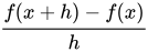
Equivalently, it is the limit as $y\rightarrow x$ of ${\frac {f(y)-f(x)}{y-x}}.$

If the derivative exists, it is commonly denoted by $f'(x)$ .

05Properties

Sequences of real numbers

For sequences of real numbers, a number of properties can be proven. Suppose $\{a_{n}\}$ and $\{b_{n}\}$ are two sequences converging to $a$ and $b$ respectively.

Sum of limits is equal to limit of sum $a_{n}+b_{n}\rightarrow a+b.$
Product of limits is equal to limit of product $a_{n}\cdot b_{n}\rightarrow a\cdot b.$
Inverse of limit is equal to limit of inverse (as long as $a\neq 0$ ) ${\frac {1}{a_{n}}}\rightarrow {\frac {1}{a}}.$

Equivalently, the function $f(x)=1/x$ is continuous about nonzero $x$ .

Cauchy sequences

A property of convergent sequences of real numbers is that they are Cauchy sequences. The definition of a Cauchy sequence $\{a_{n}\}$ is that for every real number $\varepsilon >0$ , there is an $N$ such that whenever $m,n>N$ , $|a_{m}-a_{n}|<\varepsilon .$

Informally, for any arbitrarily small error $\varepsilon$ , it is possible to find an interval of diameter $\varepsilon$ such that eventually the sequence is contained within the interval.

Cauchy sequences are closely related to convergent sequences. In fact, for sequences of real numbers they are equivalent: any Cauchy sequence is convergent.

In general metric spaces, it continues to hold that convergent sequences are also Cauchy. But the converse is not true: not every Cauchy sequence is convergent in a general metric space. A classic counterexample is the rational numbers, $\mathbb {Q}$ , with the usual distance. The sequence of decimal approximations to ${\sqrt {2}}$ , truncated at the $n$ th decimal place is a Cauchy sequence, but does not converge in $\mathbb {Q}$ .

A metric space in which every Cauchy sequence is also convergent, that is, Cauchy sequences are equivalent to convergent sequences, is known as a complete metric space.

One reason Cauchy sequences can be "easier to work with" than convergent sequences is that they are a property of the sequence $\{a_{n}\}$ alone, while convergent sequences require not just the sequence $\{a_{n}\}$ but also the limit of the sequence $a$ .

Order of convergence

Beyond whether or not a sequence $\{a_{n}\}$ converges to a limit $a$ , it is possible to describe how fast a sequence converges to a limit. One way to quantify this is using the order of convergence of a sequence.

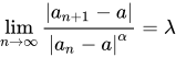
A formal definition of order of convergence can be stated as follows. Suppose $\{a_{n}\}_{n>0}$ is a sequence of real numbers which is convergent with limit $a$ . Furthermore, $a_{n}\neq a$ for all $n$ . If positive constants $\lambda$ and $\alpha$ exist such that $\lim _{n\to \infty }{\frac {\left|a_{n+1}-a\right|}{\left|a_{n}-a\right|^{\alpha }}}=\lambda$ then $a_{n}$ is said to converge to $a$ with order of convergence $\alpha$ . The constant $\lambda$ is known as the asymptotic error constant.

Order of convergence is used for example the field of numerical analysis, in error analysis.

Computability

Limits can be difficult to compute. There exist limit expressions whose modulus of convergence is undecidable. In recursion theory, the limit lemma proves that it is possible to encode undecidable problems using limits.

There are several theorems or tests that indicate whether the limit exists. These are known as convergence tests. Examples include the ratio test and the squeeze theorem. However they may not tell how to compute the limit.

Watch videos about Limit (mathematics)Explainers and documentaries on YouTube (opens in a new tab)

Sources and credits

This article is adapted from the Wikipedia article “Limit (mathematics)”, written by its contributors and licensed under CC BY-SA 4.0. Fathomly has changed the layout, removed citation markers, navigation and maintenance notices, and adjusted punctuation. This adapted version is shared under the same license. For references, see the original article.

Images, from Wikimedia Commons:

Limit-at-infinity-graph.png by Ulrik Sverdrup at English Wikipedia, CC BY-SA 3.0

Fathomly is not affiliated with or endorsed by the Wikimedia Foundation. Spotted a problem? Tell us.

Limit (mathematics)

01Notation

02History

03Types of limits

In sequences

Real numbers

Metric space

Example: ℝⁿ

Topological space

Function space

In functions

One-sided limit

Infinity in limits of functions

Nonstandard analysis

Limit sets

Limit set of a sequence

Limit set of a trajectory

04Uses

Series

Power series

Continuity of a function at a point

Continuous functions

Limit points

Derivative

05Properties

Sequences of real numbers

Cauchy sequences

Order of convergence

Computability

Sources and credits

Related topics

Asymptotic analysis

Big O notation

Banach limit

Limit (mathematics)

01Notation

02History

03Types of limits

In sequences

Real numbers

Metric space

Example: ℝn

Topological space

Function space

In functions

One-sided limit

Infinity in limits of functions

Nonstandard analysis

Limit sets

Limit set of a sequence

Limit set of a trajectory

04Uses

Series

Power series

Continuity of a function at a point

Continuous functions

Limit points

Derivative

05Properties

Sequences of real numbers

Cauchy sequences

Order of convergence

Computability

Sources and credits

Related topics

Asymptotic analysis

Big O notation

Banach limit

Example: ℝⁿ