Encyclopedia

Grover's algorithm

Quantum search algorithm

Wikipedia contributorsAdapted for Fathomly · View authors

10 min read
Source updated September 6, 2026

In quantum computing, Grover's algorithm, also known as the quantum search algorithm, is a quantum algorithm for unstructured search that finds with high probability the unique input to a black box function that produces a particular output value, using just $O({\sqrt {N}})$ evaluations of the function, where $N$ is the size of the function's domain. It was devised by an Indian-American computer scientist Lov Grover in 1996.

The analogous problem in classical computation would have a query complexity $O(N)$ (i.e., the function would have to be evaluated $O(N)$ times: there is no better approach than trying out all input values one after the other, which, on average, takes $N/2$ steps).

Charles H. Bennett, Ethan Bernstein, Gilles Brassard, and Umesh Vazirani proved that any quantum solution to the problem needs to evaluate the function $\Omega ({\sqrt {N}})$ times, so Grover's algorithm is asymptotically optimal. Since classical algorithms for NP-complete problems require exponentially many steps, and Grover's algorithm provides at most a quadratic speedup over the classical solution for unstructured search, this suggests that Grover's algorithm by itself will not provide polynomial-time solutions for NP-complete problems (as the square root of an exponential function is still an exponential, not a polynomial function).

Unlike other quantum algorithms, which may provide exponential speedup over their classical counterparts, Grover's algorithm provides only a quadratic speedup. However, even quadratic speedup is considerable when $N$ is large, and Grover's algorithm can be applied to speed up broad classes of algorithms. Grover's algorithm could brute-force a 128-bit symmetric cryptographic key in roughly 2⁶⁴ iterations, or a 256-bit key in roughly 2¹²⁸ iterations. It may not be the case that Grover's algorithm poses a significantly increased risk to encryption over existing classical algorithms, however.

01Applications and limitations

Grover's algorithm, along with variants like amplitude amplification, can be used to speed up a broad range of algorithms. In particular, algorithms for NP-complete problems which contain exhaustive search as a subroutine can be sped up by Grover's algorithm. The current theoretical best algorithm, in terms of worst-case complexity, for 3SAT is one such example. Generic constraint satisfaction problems also see quadratic speedups with Grover. These algorithms do not require that the input be given in the form of an oracle, since Grover's algorithm is being applied with an explicit function, e.g. the function checking that a set of bits satisfies a 3SAT instance. However, it is unclear whether Grover's algorithm could speed up best practical algorithms for these problems.

Grover's algorithm can also give provable speedups for black-box problems in quantum query complexity, including element distinctness and the collision problem (solved with the Brassard-Høyer-Tapp algorithm). In these types of problems, one treats the oracle function f as a database, and the goal is to use the quantum query to this function as few times as possible.

Cryptography

Grover's algorithm essentially solves the task of function inversion. Roughly speaking, if we have a function $y=f(x)$ that can be evaluated on a quantum computer, Grover's algorithm allows us to calculate $x$ when given $y$ . Consequently, Grover's algorithm gives broad asymptotic speed-ups to many kinds of brute-force attacks on symmetric-key cryptography, including collision attacks and pre-image attacks. However, this may not necessarily be the most efficient algorithm since, for example, the Pollard's rho algorithm is able to find a collision in SHA-2 more efficiently than Grover's algorithm.

Limitations

Grover's original paper described the algorithm as a database search algorithm, and this description is still common. The database in this analogy is a table of all of the function's outputs, indexed by the corresponding input. However, this database is not represented explicitly. Instead, an oracle is invoked to evaluate an item by its index. Reading a full database item by item and converting it into such a representation may take a lot longer than Grover's search. To account for such effects, Grover's algorithm can be viewed as solving an equation or satisfying a constraint. In such applications, the oracle is a way to check the constraint and is not related to the search algorithm. This separation usually prevents algorithmic optimizations, whereas conventional search algorithms often rely on such optimizations and avoid exhaustive search. Fortunately, fast Grover's oracle implementation is possible for many constraint satisfaction and optimization problems.

The major barrier to instantiating a speedup from Grover's algorithm is that the quadratic speedup achieved is too modest to overcome the large overhead of near-term quantum computers. However, later generations of fault-tolerant quantum computers with better hardware performance may be able to realize these speedups for practical instances of data.

02Problem description

As input for Grover's algorithm, suppose we have a function $f\colon \{0,1,\ldots ,N-1\}\to \{0,1\}$ . In the "unstructured database" analogy, the domain represents indices to a database, and $f(x)=1$ if the data that $x$ points to satisfies the search criterion. We additionally assume that only one index satisfies $f(x)=1$ , and we call this index $\omega$ . Our goal is to identify $\omega$ .

We can access $f$ with a subroutine (sometimes called an oracle) in the form of a unitary operator $U_{\omega }$ that acts as follows:

${\begin{cases}U_{\omega }|x\rangle =-|x\rangle &{\text{for }}x=\omega {\text{, that is, }}f(x)=1,\\U_{\omega }|x\rangle =|x\rangle &{\text{for }}x\neq \omega {\text{, that is, }}f(x)=0.\end{cases}}$

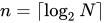
This uses the $N$ -dimensional state space ${\mathcal {H}}$ , which is supplied by a register with $n=\lceil \log _{2}N\rceil$ qubits. This is often written as

$U_{\omega }|x\rangle =(-1)^{f(x)}|x\rangle .$

Grover's algorithm outputs $\omega$ with probability at least $1/2$ using $O({\sqrt {N}})$ applications of $U_{\omega }$ . This probability can be made arbitrarily large by running Grover's algorithm multiple times. If one runs Grover's algorithm until $\omega$ is found, the expected number of applications is still $O({\sqrt {N}})$ , since it will only be run twice on average.

Alternative oracle definition

This section compares the above oracle $U_{\omega }$ with an oracle $U_{f}$ .

$U_{\omega }$ is different from the standard quantum oracle for a function $f$ . This standard oracle, denoted here as $U_{f}$ , uses an ancillary qubit system. The operation then represents an inversion (NOT gate) on the main system conditioned by the value of f(x) from the ancillary system:

${\begin{cases}U_{f}|x\rangle |y\rangle =|x\rangle |\neg y\rangle &{\text{for }}x=\omega {\text{, that is, }}f(x)=1,\\U_{f}|x\rangle |y\rangle =|x\rangle |y\rangle &{\text{for }}x\neq \omega {\text{, that is, }}f(x)=0,\end{cases}}$

or briefly,

$U_{f}|x\rangle |y\rangle =|x\rangle |y\oplus f(x)\rangle .$

These oracles are typically realized using uncomputation.

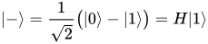
If we are given $U_{f}$ as our oracle, then we can also implement $U_{\omega }$ , since $U_{\omega }$ is $U_{f}$ when the ancillary qubit is in the state $|-\rangle ={\frac {1}{\sqrt {2}}}{\big (}|0\rangle -|1\rangle {\big )}=H|1\rangle$ :

${\begin{aligned}U_{f}{\big (}|x\rangle \otimes |-\rangle {\big )}&={\frac {1}{\sqrt {2}}}\left(U_{f}|x\rangle |0\rangle -U_{f}|x\rangle |1\rangle \right)\\&={\frac {1}{\sqrt {2}}}\left(|x\rangle |0\oplus f(x)\rangle -|x\rangle |1\oplus f(x)\rangle \right)\\&={\begin{cases}{\frac {1}{\sqrt {2}}}\left(-|x\rangle |0\rangle +|x\rangle |1\rangle \right)&{\text{if }}f(x)=1,\\{\frac {1}{\sqrt {2}}}\left(|x\rangle |0\rangle -|x\rangle |1\rangle \right)&{\text{if }}f(x)=0\end{cases}}\\&=(U_{\omega }|x\rangle )\otimes |-\rangle \end{aligned}}$

So, Grover's algorithm can be run regardless of which oracle is given. If $U_{f}$ is given, then we must maintain an additional qubit in the state $|-\rangle$ and apply $U_{f}$ in place of $U_{\omega }$ .

03Algorithm

The steps of Grover's algorithm are given as follows:

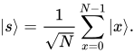
Initialize the system to the uniform superposition over all states
$|s\rangle ={\frac {1}{\sqrt {N}}}\sum _{x=0}^{N-1}|x\rangle .$
Perform the following "Grover iteration" times:
1. Apply the operator $U_{\omega }$
2. Apply the Grover diffusion operator $U_{s}=2\left|s\right\rangle \!\!\left\langle s\right|-I$
Measure the resulting quantum state in the computational basis.

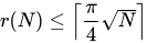
For the correctly chosen value of $r$ , the output will be $|\omega \rangle$ with probability approaching 1 for N ≫ 1. Analysis shows that this eventual value for $r(N)$ satisfies $r(N)\leq {\Big \lceil }{\frac {\pi }{4}}{\sqrt {N}}{\Big \rceil }$ .

Implementing the steps for this algorithm can be done using a number of gates linear in the number of qubits. Thus, the gate complexity of this algorithm is $O(\log(N)r(N))$ , or $O(\log(N))$ per iteration.

04Geometric proof

There is a geometric interpretation of Grover's algorithm, following from the observation that the quantum state of Grover's algorithm stays in a two-dimensional subspace after each step. Consider the plane spanned by $|s\rangle$ and $|\omega \rangle$ ; equivalently, the plane spanned by $|\omega \rangle$ and the perpendicular ket $\textstyle |s'\rangle ={\frac {1}{\sqrt {N-1}}}\sum _{x\neq \omega }|x\rangle$ .

Grover's algorithm begins with the initial ket $|s\rangle$ , which lies in the subspace. The operator $U_{\omega }$ is a reflection at the hyperplane orthogonal to $|\omega \rangle$ for vectors in the plane spanned by $|s'\rangle$ and $|\omega \rangle$ , i.e. it acts as a reflection across $|s'\rangle$ . This can be seen by writing $U_{\omega }$ in the form of a Householder reflection:

$U_{\omega }=I-2|\omega \rangle \langle \omega |.$

The operator $U_{s}=2|s\rangle \langle s|-I$ is a reflection through $|s\rangle$ . Both operators $U_{s}$ and $U_{\omega }$ take states in the plane spanned by $|s'\rangle$ and $|\omega \rangle$ to states in the plane. Therefore, Grover's algorithm stays in this plane for the entire algorithm.

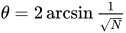
It is straightforward to check that the operator $U_{s}U_{\omega }$ of each Grover iteration step rotates the state vector by an angle of $\theta =2\arcsin {\tfrac {1}{\sqrt {N}}}$ . So, with enough iterations, one can rotate from the initial state $|s\rangle$ to the desired output state $|\omega \rangle$ . The initial ket is close to the state orthogonal to $|\omega \rangle$ :

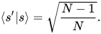
$\langle s'|s\rangle ={\sqrt {\frac {N-1}{N}}}.$

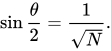
In geometric terms, the angle $\theta /2$ between $|s\rangle$ and $|s'\rangle$ is given by

$\sin {\frac {\theta }{2}}={\frac {1}{\sqrt {N}}}.$

We need to stop when the state vector passes close to $|\omega \rangle$ ; after this, subsequent iterations rotate the state vector away from $|\omega \rangle$ , reducing the probability of obtaining the correct answer. The exact probability of measuring the correct answer is

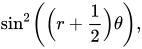
$\sin ^{2}\left({\Big (}r+{\frac {1}{2}}{\Big )}\theta \right),$

where r is the (integer) number of Grover iterations. The earliest time that we get a near-optimal measurement is therefore $r\approx \pi {\sqrt {N}}/4$ .

05Algebraic proof

To complete the algebraic analysis, we need to find out what happens when we repeatedly apply $U_{s}U_{\omega }$ . A natural way to do this is by eigenvalue analysis of a matrix. Notice that during the entire computation, the state of the algorithm is a linear combination of $s$ and $\omega$ . We can write the action of $U_{s}$ and $U_{\omega }$ in the space spanned by $\{|s\rangle ,|\omega \rangle \}$ as:

${\begin{aligned}U_{s}:a|\omega \rangle +b|s\rangle &\mapsto [|\omega \rangle \,|s\rangle ]{\begin{bmatrix}-1&0\\2/{\sqrt {N}}&1\end{bmatrix}}{\begin{bmatrix}a\\b\end{bmatrix}}.\\U_{\omega }:a|\omega \rangle +b|s\rangle &\mapsto [|\omega \rangle \,|s\rangle ]{\begin{bmatrix}-1&-2/{\sqrt {N}}\\0&1\end{bmatrix}}{\begin{bmatrix}a\\b\end{bmatrix}}.\end{aligned}}$

So in the basis $\{|\omega \rangle ,|s\rangle \}$ (which is neither orthogonal nor a basis of the whole space) the action $U_{s}U_{\omega }$ of applying $U_{\omega }$ followed by $U_{s}$ is given by the matrix

$U_{s}U_{\omega }={\begin{bmatrix}-1&0\\2/{\sqrt {N}}&1\end{bmatrix}}{\begin{bmatrix}-1&-2/{\sqrt {N}}\\0&1\end{bmatrix}}={\begin{bmatrix}1&2/{\sqrt {N}}\\-2/{\sqrt {N}}&1-4/N\end{bmatrix}}.$

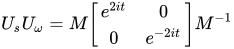
This matrix happens to have a very convenient Jordan form. If we define $t=\arcsin(1/{\sqrt {N}})$ , it is

$U_{s}U_{\omega }=M{\begin{bmatrix}e^{2it}&0\\0&e^{-2it}\end{bmatrix}}M^{-1}$

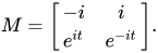
where $M={\begin{bmatrix}-i&i\\e^{it}&e^{-it}\end{bmatrix}}.$

It follows that r-th power of the matrix (corresponding to r iterations) is

$(U_{s}U_{\omega })^{r}=M{\begin{bmatrix}e^{2rit}&0\\0&e^{-2rit}\end{bmatrix}}M^{-1}.$

Using this form, we can use trigonometric identities to compute the probability of observing ω after r iterations mentioned in the previous section,

$\left|{\begin{bmatrix}\langle \omega |\omega \rangle &\langle \omega |s\rangle \end{bmatrix}}(U_{s}U_{\omega })^{r}{\begin{bmatrix}0\\1\end{bmatrix}}\right|^{2}=\sin ^{2}\left((2r+1)t\right).$

Alternatively, one might reasonably imagine that a near-optimal time to distinguish would be when the angles 2rt and −2rt are as far apart as possible, which corresponds to $2rt\approx \pi /2$ , or $r=\pi /4t=\pi /4\arcsin(1/{\sqrt {N}})\approx \pi {\sqrt {N}}/4$ . Then the system is in state

$[|\omega \rangle \,|s\rangle ](U_{s}U_{\omega })^{r}{\begin{bmatrix}0\\1\end{bmatrix}}\approx [|\omega \rangle \,|s\rangle ]M{\begin{bmatrix}i&0\\0&-i\end{bmatrix}}M^{-1}{\begin{bmatrix}0\\1\end{bmatrix}}=|\omega \rangle {\frac {1}{\cos(t)}}-|s\rangle {\frac {\sin(t)}{\cos(t)}}.$

A short calculation now shows that the observation yields the correct answer ω with error $O\left({\frac {1}{N}}\right)$ .

06Extensions and variants

Multiple matching entries

If, instead of 1 matching entry, there are k matching entries, the same algorithm works, but the number of iterations must be ${\textstyle {\frac {\pi }{4}}{\sqrt {\frac {N}{k}}}$ instead of ${\textstyle {\frac {\pi }{4}}{\sqrt {N}}$ .

There are several ways to handle the case if k is unknown. A simple solution performs optimally up to a constant factor: run Grover's algorithm repeatedly for increasingly small values of k, e.g., taking k = N, N/2, N/4, ..., and so on, taking $k=N/2^{t}$ for iteration t until a matching entry is found.

With sufficiently high probability, a marked entry will be found by iteration $t=\log _{2}(N/k)+c$ for some constant c. Thus, the total number of iterations taken is at most

${\frac {\pi }{4}}{\Big (}1+{\sqrt {2}}+{\sqrt {4}}+\cdots +{\sqrt {\frac {N}{k2^{c}}}}{\Big )}=O{\big (}{\sqrt {N/k}}{\big )}.$

Another approach if k is unknown is to derive it via the quantum counting algorithm prior.

If $k=N/2$ (or the traditional one marked state Grover's Algorithm if run with $N=2$ ), the algorithm will provide no amplification. If $k>N/2$ , increasing k will begin to increase the number of iterations necessary to obtain a solution. On the other hand, if $k\geq N/2$ , a classical running of the checking oracle on a single random choice of input will more likely than not give a correct solution.

A version of this algorithm is used in order to solve the collision problem.

Quantum partial search

A modification of Grover's algorithm called quantum partial search was described by Grover and Radhakrishnan in 2004. In partial search, one is not interested in finding the exact address of the target item, only the first few digits of the address. Equivalently, we can think of "chunking" the search space into blocks, and then asking "in which block is the target item?". In many applications, such a search yields enough information if the target address contains the information wanted. For instance, to use the example given by L. K. Grover, if one has a list of students organized by class rank, we may only be interested in whether a student is in the lower 25%, 25-50%, 50-75% or 75-100% percentile.

To describe partial search, we consider a database separated into $K$ blocks, each of size $b=N/K$ . The partial search problem is easier. Consider the approach we would take classically, we pick one block at random, and then perform a normal search through the rest of the blocks (in set theory language, the complement). If we do not find the target, then we know it is in the block we did not search. The average number of iterations drops from $N/2$ to $(N-b)/2$ .

Grover's algorithm requires ${\textstyle {\frac {\pi }{4}}{\sqrt {N}}$ iterations. Partial search will be faster by a numerical factor that depends on the number of blocks $K$ . Partial search uses $n_{1}$ global iterations and $n_{2}$ local iterations. The global Grover operator is designated $G_{1}$ and the local Grover operator is designated $G_{2}$ .

The global Grover operator acts on the blocks. Essentially, it is given as follows:

Perform $j_{1}$ standard Grover iterations on the entire database.
Perform $j_{2}$ local Grover iterations. A local Grover iteration is a direct sum of Grover iterations over each block.
Perform one standard Grover iteration.

The optimal values of $j_{1}$ and $j_{2}$ are discussed in the paper by Grover and Radhakrishnan. One might also wonder what happens if one applies successive partial searches at different levels of "resolution". This idea was studied in detail by Vladimir Korepin and Xu, who called it binary quantum search. They proved that it is not in fact any faster than performing a single partial search.

07Optimality

Grover's algorithm is optimal up to sub-constant factors. That is, any algorithm that accesses the database only by using the operator U_ω must apply U_ω at least a $1-o(1)$ fraction as many times as Grover's algorithm. The extension of Grover's algorithm to k matching entries, π(N/k)^1/2/4, is also optimal. This result is important in understanding the limits of quantum computation.

If the Grover's search problem was solvable with log^c N applications of U_ω, that would imply that NP is contained in BQP, by transforming problems in NP into Grover-type search problems. The optimality of Grover's algorithm suggests that quantum computers cannot solve NP-Complete problems in polynomial time, and thus NP is not contained in BQP.

It has been shown that a class of non-local hidden variable quantum computers could implement a search of an $N$ -item database in at most $O({\sqrt[{3}]{N}})$ steps. This is faster than the $O({\sqrt {N}})$ steps taken by Grover's algorithm.

Watch videos about Grover's algorithmExplainers and documentaries on YouTube (opens in a new tab)

Sources and credits

This article is adapted from the Wikipedia article “Grover's algorithm”, written by its contributors and licensed under CC BY-SA 4.0. Fathomly has changed the layout, removed citation markers, navigation and maintenance notices, and adjusted punctuation. This adapted version is shared under the same license. For references, see the original article.

Images, from Wikimedia Commons:

Grover's algorithm circuit.svg by Fawly, CC BY-SA 4.0
Grovers algorithm geometry.png by Danski14, CC BY-SA 3.0

Fathomly is not affiliated with or endorsed by the Wikimedia Foundation. Spotted a problem? Tell us.