Encyclopedia

Chebyshev polynomials

Pair of polynomial sequences

Wikipedia contributorsAdapted for Fathomly · View authors

15 min read
Source updated April 27, 2026

The Chebyshev polynomials are two sequences of orthogonal polynomials related to the cosine and sine functions, notated as $T_{n}(x)$ and $U_{n}(x)$ . They can be defined in several equivalent ways, one of which starts with trigonometric functions:

The Chebyshev polynomials of the first kind $T_{n}$ are defined by

$T_{n}(\cos \theta )=\cos(n\theta ).$

Similarly, the Chebyshev polynomials of the second kind $U_{n}$ are defined by

$U_{n}(\cos \theta )\sin \theta ={\sin }{\big (}(n+1)\theta {\big )}.$

That these expressions define polynomials in $\cos \theta$ is not obvious at first sight but can be shown using de Moivre's formula (see below).

The Chebyshev polynomials T_n are polynomials with the largest possible leading coefficient whose absolute value on the interval [−1, 1] is bounded by 1. They are also the "extremal" polynomials for many other properties.

In 1952, Cornelius Lanczos showed that the Chebyshev polynomials are important in approximation theory for the solution of linear systems; the roots of T_n(x), which are also called Chebyshev nodes, are used as matching points for optimizing polynomial interpolation. The resulting interpolation polynomial minimizes the problem of Runge's phenomenon and provides an approximation that is close to the best polynomial approximation to a continuous function under the maximum norm, also called the "minimax" criterion. This approximation leads directly to the method of Clenshaw-Curtis quadrature.

These polynomials were named after Pafnuty Chebyshev. The letter T is used because of the alternative transliterations of the name Chebyshev as Tchebycheff, Tchebyshev (French) or Tschebyschow (German).

01Definitions

Recurrence definition

The Chebyshev polynomials of the first kind can be defined by the recurrence relation

${\begin{aligned}T_{0}(x)&=1,\\T_{1}(x)&=x,\\T_{n+1}(x)&=2x\,T_{n}(x)-T_{n-1}(x).\end{aligned}}$

The Chebyshev polynomials of the second kind can be defined by the recurrence relation

${\begin{aligned}U_{0}(x)&=1,\\U_{1}(x)&=2x,\\U_{n+1}(x)&=2x\,U_{n}(x)-U_{n-1}(x),\end{aligned}}$ which differs from the above only by the rule for n=1.

Trigonometric definition

The Chebyshev polynomials of the first and second kind can be defined as the unique polynomials satisfying $T_{n}(\cos \theta )=\cos(n\theta )\quad$ and $U_{n}(\cos \theta )={\frac {{\sin }{\big (}(n+1)\theta {\big )}}{\sin \theta }},$ for n = 0, 1, 2, 3, ….

An equivalent way to state this is via exponentiation of a complex number: given a complex number z = a + bi with absolute value of one, $z^{n}=T_{n}(a)+ib\,U_{n-1}(a).$

Chebyshev polynomials can also be defined in this form when studying trigonometric polynomials.

That $\cos(nx)$ is an $n$ th-degree polynomial in $\cos(x)$ can be seen by observing that $\cos(nx)$ is the real part of one side of de Moivre's formula: $\cos n\theta +i\sin n\theta =(\cos \theta +i\sin \theta )^{n}.$

The real part of the other side is a polynomial in $\cos x$ and $\sin x$ , in which all powers of $\sin x$ are even and thus replaceable through the identity $\cos ^{2}x+\sin ^{2}x=1$ . By the same reasoning, $\sin nx$ is the imaginary part of the polynomial, in which all powers of $\sin x$ are odd and thus, if one factor of $\sin x$ is factored out, the remaining factors can be replaced to create a polynomial of degree $n-1$ in $\cos x$ .

For $x$ outside the interval [-1,1], the above definition implies $T_{n}(x)={\begin{cases}\cos(n\arccos x)&{\text{ if }}|x|\leq 1,\\\cosh(n\operatorname {arccosh} x)&{\text{ if }}x\geq 1,\\{(-1)^{n}\cosh }(n\operatorname {arccosh} (-x))&{\text{ if }}x\leq -1.\end{cases}}$

Commuting polynomials definition

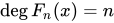
Chebyshev polynomials can also be characterized by the following theorem:

If $F_{n}(x)$ is a family of monic polynomials with coefficients in a field of characteristic $0$ such that $\deg F_{n}(x)=n$ and $F_{m}{\bigl (}F_{n}(x){\bigr )}=F_{n}{\bigl (}F_{m}(x){\bigr )}$ for all $m$ and $n$ , then, up to a simple change of variables, either $F_{n}(x)=x^{n}$ for all $n$ or $F_{n}(x)=2\cdot T_{n}{\bigl (}{\tfrac {1}{2}}x{\bigr )}$ for all $n$ .

Pell equation definition

The Chebyshev polynomials can also be defined as the solutions to the Pell equation: $T_{n}(x)^{2}-(x^{2}-1)\,U_{n-1}(x)^{2}=1$

in a ring ⁠ $R[x]$ ⁠. Thus, they can be generated by the standard technique for Pell equations of taking powers of a fundamental solution: $T_{n}(x)+U_{n-1}(x){\textstyle {\sqrt {x^{2}-1}}}={\bigl (}{\textstyle x+{\sqrt {x^{2}-1}}~\!}{\bigr )}^{n}.$

Generating functions

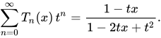
The ordinary generating function for $T_{n}$ is $\sum _{n=0}^{\infty }T_{n}(x)\,t^{n}={\frac {1-tx}{1-2tx+t^{2}}}.$

There are several other generating functions for the Chebyshev polynomials; the exponential generating function is ${\begin{aligned}\sum _{n=0}^{\infty }T_{n}(x){\frac {t^{n}}{n!}}&={\tfrac {1}{2}}{\Bigl (}{\exp }{\Bigl (}t{\bigl (}{\textstyle x-{\sqrt {x^{2}-1}}~\!}{\bigr )}{\Bigr )}+{\exp }{\Bigl (}t{\bigl (}{\textstyle x+{\sqrt {x^{2}-1}}~\!}{\bigr )}{\Bigr )}{\Bigr )}\\&={e^{tx}\cosh }{\bigl (}{\textstyle t{\sqrt {x^{2}-1}}}~\!{\bigr )}.\end{aligned}}$

The generating function relevant for 2-dimensional potential theory and multipole expansion is $\sum \limits _{n=1}^{\infty }T_{n}(x){\frac {t^{n}}{n}}=\ln \left({\frac {1}{\sqrt {1-2tx+t^{2}}}}\right).$

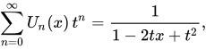
The ordinary generating function for U_n is $\sum _{n=0}^{\infty }U_{n}(x)\,t^{n}={\frac {1}{1-2tx+t^{2}}},$ and the exponential generating function is $\sum _{n=0}^{\infty }U_{n}(x){\frac {t^{n}}{n!}}=e^{tx}{\biggl (}{\cosh }{\bigl (}{\textstyle t{\sqrt {x^{2}-1}}~\!}{\bigr )}+{{\frac {x}{\sqrt {x^{2}-1}}}\sinh }{\bigl (}{\textstyle t{\sqrt {x^{2}-1}}~\!}{\bigr )}{\biggr )}.$

02Relations between the two kinds of Chebyshev polynomials

The Chebyshev polynomials of the first and second kinds correspond to a complementary pair of Lucas sequences ${\tilde {V}}_{n}(P,Q)$ and ${\tilde {U}}_{n}(P,Q)$ with parameters $P=2x$ and $Q=1$ :

${\begin{aligned}{\tilde {U}}_{n}(2x,1)&=U_{n-1}(x),\\{\tilde {V}}_{n}(2x,1)&=2\,T_{n}(x).\end{aligned}}$

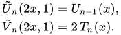
It follows that they also satisfy a pair of mutual recurrence equations:

${\begin{aligned}T_{n+1}(x)&=x\,T_{n}(x)-(1-x^{2})\,U_{n-1}(x),\\U_{n+1}(x)&=x\,U_{n}(x)+T_{n+1}(x).\end{aligned}}$

The second of these may be rearranged using the recurrence definition for the Chebyshev polynomials of the second kind to give: $T_{n}(x)={\tfrac {1}{2}}{\big (}U_{n}(x)-U_{n-2}(x){\big )}.$

Using this formula iteratively gives the sum formula: $U_{n}(x)={\begin{cases}2\sum _{{\text{ odd }}j>0}^{n}T_{j}(x)&{\text{ for odd }}n.\\2\sum _{{\text{ even }}j\geq 0}^{n}T_{j}(x)-1&{\text{ for even }}n,\end{cases}}$

while replacing $U_{n}(x)$ and $U_{n-2}(x)$ using the derivative formula for $T_{n}(x)$ gives the recurrence relationship for the derivative of $T_{n}$ : $2T_{n}(x)={\frac {1}{n+1}},{\frac {\mathrm {d} }{\mathrm {d} x}}\,T_{n+1}(x)-{\frac {1}{n-1}}\,{\frac {\mathrm {d} }{\mathrm {d} x}}\,T_{n-1}(x),$ for $n=2,3,\ldots$ .

This relationship is used in the Chebyshev spectral method of solving differential equations.

Turán's inequalities for the Chebyshev polynomials are: ${\begin{aligned}T_{n}(x)^{2}-T_{n-1}(x)\,T_{n+1}(x)&=1-x^{2}>0&&{\text{ for }}-1<x<1&&{\text{ and }}\\U_{n}(x)^{2}-U_{n-1}(x)\,U_{n+1}(x)&=1>0.\end{aligned}}$

The integral relations are ${\begin{aligned}\int _{-1}^{1}{\frac {T_{n}(y)}{y-x}}\,{\frac {\mathrm {d} y}{\sqrt {1-y^{2}}}}&=\pi \,U_{n-1}(x),\\[3mu]\int _{-1}^{1}{\frac {U_{n-1}(y)}{y-x}}\,{\textstyle {\sqrt {1-y^{2}}}}\,\mathrm {d} y&=-\pi \,T_{n}(x)\end{aligned}}$

where integrals are considered as principal value.

03Explicit expressions

Using the complex number exponentiation definition of the Chebyshev polynomial, one can derive the following expressions, valid for any real ⁠ $x$ ⁠: ${\begin{aligned}T_{n}(x)&={\tfrac {1}{2}}{\Bigl (}{\bigl (}{\textstyle x-{\sqrt {x^{2}-1}}\!~}{\bigr )}^{n}+{\bigl (}{\textstyle x+{\sqrt {x^{2}-1}}\!~}{\bigr )}^{n}{\Bigr )}\\[5mu]&={\tfrac {1}{2}}{\Bigl (}{\bigl (}{\textstyle x-{\sqrt {x^{2}-1}}\!~}{\bigr )}^{n}+{\bigl (}{\textstyle x-{\sqrt {x^{2}-1}}\!~}{\bigr )}^{-n}{\Bigr )}.\end{aligned}}$ The two are equivalent because $\textstyle {\bigl (}x+{\sqrt {x^{2}-1}}\!~{\bigr )}^{\pm 1}={\bigl (}x-{\sqrt {x^{2}-1}}\!~{\bigr )}^{\mp 1}.$

An explicit form of the Chebyshev polynomial in terms of monomials $\textstyle x^{k}$ can be obtained as follows. Letting ${\mathfrak {R}}$ denote the real part of a complex number, the following equalities, in order, follow by the definition of $T_{n}$ , the definition of ${\mathfrak {R}}$ , de Moivre's formula, and the binomial theorem: ${\begin{aligned}T_{n}{\bigl (}\cos(\theta ){\bigr )}&=\cos(n\theta )\\&={\mathfrak {R}}{\bigl (}\cos(n\theta )+i\sin(n\theta ){\bigr )}\\&={\mathfrak {R}}{\bigl (}(\cos(\theta )+i\sin(\theta ))^{n}{\bigr )}\\&={\mathfrak {R}}\left(\sum _{j=0}^{n}{\binom {n}{j}}\,i^{j}\sin ^{j}(\theta )\,\cos ^{n-j}(\theta )\right).\end{aligned}}$ Because of the factor of $i^{j}$ , the even-indexed terms are purely real, while the odd-indexed terms are purely imaginary; furthermore, $\sin ^{2j}\theta =\left(1-\cos ^{2}\theta \right)^{j},$ so $T_{n}{\bigl (}\cos(\theta ){\bigr )}=\sum _{j=0}^{\lfloor n/2\rfloor }{\binom {n}{2j}}\,(-1)^{j}(1-\cos ^{2}(\theta ))^{j}\cos ^{n-2j}(\theta ).$ Finally, substituting $x=\cos(\theta )$ yields $T_{n}(x)=\sum \limits _{j=0}^{\lfloor n/2\rfloor }{\binom {n}{2j}}\left(x^{2}-1\right)^{j}x^{n-2j}.$ This can be written as a ⁠ ${}_{2}F_{1}$ ⁠ hypergeometric function: ${\begin{aligned}T_{n}(x)&=\sum _{k=0}^{\lfloor n/2\rfloor }{\binom {n}{2k}}(x^{2}-1)^{k}x^{n-2k}\\&=x^{n}\sum _{k=0}^{\lfloor n/2\rfloor }{\binom {n}{2k}}(1-x^{-2})^{k}\\&={\tfrac {1}{2}}n\sum _{k=0}^{\lfloor n/2\rfloor }(-1)^{k}{\frac {(n-k-1)!}{k!(n-2k)!}}(2x)^{n-2k}\qquad {\text{ for }}n>0\\&=n\sum _{k=0}^{n}(-2)^{k}{\frac {(n+k-1)!}{(n-k)!(2k)!}}(1-x)^{k}\qquad {\text{ for }}n>0\\&={}_{2}F_{1}{\bigl (}{-n},n;{\tfrac {1}{2}};{\tfrac {1}{2}}(1-x){\bigr )}\\\end{aligned}}$ with inverse $x^{n}={\frac {1}{2^{n-1}}}\mathop {{\sum }'} _{{j=0} \atop {j\equiv n{\pmod {2}}}}^{n}{\binom {n}{\tfrac {n-j}{2}}}T_{j}(x),$ where the prime on the summation symbol indicates that the contribution of $j=0$ needs to be halved if it appears.

A related expression for $T_{n}$ as a sum of monomials with binomial coefficients and powers of two is $T_{n}(x)=\sum \limits _{m=0}^{\lfloor n/2\rfloor }(-1)^{m}{\Biggl (}{\binom {n-m}{m}}+{\binom {n-m-1}{n-2m}}{\Biggr )}\cdot 2^{n-2m-1}\cdot x^{n-2m}.$ Similarly, $U_{n}$ can be expressed in terms of hypergeometric functions: ${\begin{aligned}U_{n}(x)&={\frac {{\bigl (}x+{\sqrt {x^{2}-1}}~\!{\bigr )}^{n+1}-{\bigl (}x-{\sqrt {x^{2}-1}}~\!{\bigr )}^{n+1}}{2{\sqrt {x^{2}-1}}}}\\&=\sum _{k=0}^{\lfloor n/2\rfloor }{\binom {n+1}{2k+1}}{\bigl (}x^{2}-1{\bigr )}^{k}x^{n-2k}\\&=x^{n}\sum _{k=0}^{\lfloor n/2\rfloor }{\binom {n+1}{2k+1}}{\bigl (}1-x^{-2}{\bigr )}^{k}\\&=\sum _{k=0}^{\lfloor n/2\rfloor }{\binom {2k-(n+1)}{k}}(2x)^{n-2k}&{\text{ for }}n>0\\&=\sum _{k=0}^{\lfloor n/2\rfloor }(-1)^{k}{\binom {n-k}{k}}(2x)^{n-2k}&{\text{ for }}n>0\\&=\sum _{k=0}^{n}(-2)^{k}{\frac {(n+k+1)!}{(n-k)!(2k+1)!}}(1-x)^{k}&{\text{ for }}n>0\\&=(n+1)\cdot {}_{2}F_{1}{\bigl (}{-n},n+2;{\tfrac {3}{2}};{\tfrac {1}{2}}(1-x){\bigr )}.\end{aligned}}$

04Properties

Symmetry

${\begin{aligned}T_{n}(-x)&=(-1)^{n}T_{n}(x),\\[1ex]U_{n}(-x)&=(-1)^{n}U_{n}(x).\end{aligned}}$ That is, Chebyshev polynomials of even order have even symmetry and therefore contain only even powers of $x$ . Chebyshev polynomials of odd order have odd symmetry and therefore contain only odd powers of $x$ .

Roots and extrema

A Chebyshev polynomial of either kind with degree n has n different simple roots, called Chebyshev roots, in the interval [−1, 1]. The roots of the Chebyshev polynomial of the first kind are sometimes called Chebyshev nodes because they are used as nodes in polynomial interpolation. Using the trigonometric definition and the fact that $\cos \left((2k+1){\frac {\pi }{2}}\right)=0,$ one can show that the roots of $T_{n}$ are $x_{k}=\cos \left({\frac {2k+1}{2n}}\pi \right),\quad k=0,\ldots ,n-1.$ Similarly, the roots of $U_{n}$ are: $x_{k}=\cos \left({\frac {k}{n+1}}\pi \right),\quad k=1,\ldots ,n.$ The extrema of $T_{n}$ on the interval $-1\leq x\leq 1$ are located at: $x_{k}=\cos \left({\frac {k}{n}}\pi \right),\quad k=0,\ldots ,n.$ One unique property of the Chebyshev polynomials of the first kind is that on the interval $-1\leq x\leq 1$ all of the extrema have values that are either −1 or 1. Thus these polynomials have only two finite critical values, the defining property of Shabat polynomials. Both the first and second kinds of Chebyshev polynomial have extrema at the endpoints, given by: ${\begin{aligned}T_{n}(1)&=1\\T_{n}(-1)&=(-1)^{n}\\U_{n}(1)&=n+1\\U_{n}(-1)&=(-1)^{n}(n+1).\end{aligned}}$ The extrema of $T_{n}(x)$ on the interval $-1\leq x\leq 1$ where $n>0$ are located at $n+1$ values of $x$ . They are $\pm 1$ , or $\cos(2\pi k/d)$ where $d>2$ , $d\mid 2n$ , $0<k<{\tfrac {1}{2}}d$ and $(k,d)=1$ , i.e., $k$ and $d$ are relatively prime.

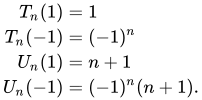
Specifically (Minimal polynomial of 2cos(2pi/n)) when $n$ is even:

$T_{n}(x)=1$ if $x=\pm 1$ , or $d>2$ and $2n/d$ is even. There are ${\tfrac {1}{2}}n+1$ such values of $x$ .
$T_{n}(x)=-1$ if $d>2$ and $2n/d$ is odd. There are ${\tfrac {1}{2}}n$ such values of $x$ .

When $n$ is odd:

$T_{n}(x)=1$ if $x=1$ , or $d>2$ and $2n/d$ is even. There are ${\tfrac {1}{2}}(n+1)$ such values of $x$ .
$T_{n}(x)=-1$ if $x=-1$ , or $d>2$ and $2n/d$ is odd. There are ${\tfrac {1}{2}}(n+1)$ such values of $x$ .

Differentiation and integration

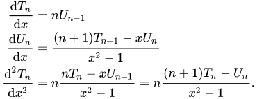
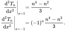
The derivatives of the polynomials can be less than straightforward. By differentiating the polynomials in their trigonometric forms, it can be shown that: ${\begin{aligned}{\frac {\mathrm {d} T_{n}}{\mathrm {d} x}}&=nU_{n-1}\\{\frac {\mathrm {d} U_{n}}{\mathrm {d} x}}&={\frac {(n+1)T_{n+1}-xU_{n}}{x^{2}-1}}\\{\frac {\mathrm {d} ^{2}T_{n}}{\mathrm {d} x^{2}}}&=n{\frac {nT_{n}-xU_{n-1}}{x^{2}-1}}=n{\frac {(n+1)T_{n}-U_{n}}{x^{2}-1}}.\end{aligned}}$ The last two formulas can be numerically troublesome due to the division by zero (⁠0/0⁠ indeterminate form, specifically) at $x=1$ and $x=-1$ . By L'Hôpital's rule: ${\begin{aligned}\left.{\frac {\mathrm {d} ^{2}T_{n}}{\mathrm {d} x^{2}}}\right|_{x=1}\!\!&={\frac {n^{4}-n^{2}}{3}},\\\left.{\frac {\mathrm {d} ^{2}T_{n}}{\mathrm {d} x^{2}}}\right|_{x=-1}\!\!&=(-1)^{n}{\frac {n^{4}-n^{2}}{3}}.\end{aligned}}$ More generally, $\left.{\frac {\mathrm {d} ^{p}T_{n}}{\mathrm {d} x^{p}}}\right|_{x=\pm 1}\!\!=(\pm 1)^{n+p}\prod _{k=0}^{p-1}{\frac {n^{2}-k^{2}}{2k+1}},$ which is of great use in the numerical solution of eigenvalue problems.

Also, we have: ${\frac {\mathrm {d} ^{p}}{\mathrm {d} x^{p}}}T_{n}(x)=2^{p}n\mathop {{\sum }'} _{0\leq k\leq n-p \atop k\equiv n-p{\pmod {2}}}{\binom {{\frac {n+p-k}{2}}-1}{\frac {n-p-k}{2}}}{\frac {\left({\frac {n+p+k}{2}}-1\right)!}{\left({\frac {n-p+k}{2}}\right)!}}T_{k}(x),\qquad p\geq 1,$ where the prime at the summation symbols means that the term contributed by k = 0 is to be halved, if it appears.

Concerning integration, the first derivative of the T_n implies that: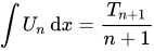 $\int U_{n}\,\mathrm {d} x={\frac {T_{n+1}}{n+1}}$ and the recurrence relation for the first kind polynomials involving derivatives establishes that for $n\geq 2$ : $\int T_{n}\,\mathrm {d} x={\frac {1}{2}}\left({\frac {T_{n+1}}{n+1}}-{\frac {T_{n-1}}{n-1}}\right)={\frac {n\,T_{n+1}}{n^{2}-1}}-{\frac {xT_{n}}{n-1}}.$ The last formula can be further manipulated to express the integral of $T_{n}$ as a function of Chebyshev polynomials of the first kind only: ${\begin{aligned}\int T_{n}\,\mathrm {d} x&={\frac {n}{n^{2}-1}}T_{n+1}-{\frac {1}{n-1}}T_{1}T_{n}\\&={\frac {n}{n^{2}-1}}T_{n+1}-{\frac {1}{2(n-1)}}(T_{n+1}+T_{n-1})\\&={\frac {1}{2(n+1)}}T_{n+1}-{\frac {1}{2(n-1)}}T_{n-1}.\end{aligned}}$ Furthermore, we have: $\int _{-1}^{1}T_{n}(x)\,\mathrm {d} x={\begin{cases}{\dfrac {(-1)^{n}+1}{1-n^{2}}}&{\text{ if }}n\neq 1\\[3mu]0&{\text{ if }}n=1.\end{cases}}$

Products of Chebyshev polynomials

The Chebyshev polynomials of the first kind satisfy the relation $T_{m}(x)\,T_{n}(x)={\tfrac {1}{2}}{\left(T_{m+n}(x)+T_{|m-n|}(x)\right)},$ for all non-negative values of ⁠ $m$ ⁠ and ⁠ $n$ ⁠, which is easily proved from the product-to-sum formula for the cosine: $2\cos \alpha \,\cos \beta =\cos(\alpha +\beta )+\cos(\alpha -\beta ).$ For $n=1$ this results in the already-known recurrence formula, just arranged differently, and with $n=2$ it forms the recurrence relation for all even or all odd indexed Chebyshev polynomials (depending on the parity of the lowest m) which implies the evenness or oddness of these polynomials. Three more useful formulas for evaluating Chebyshev polynomials can be concluded from this product expansion: ${\begin{aligned}T_{2n}(x)&=2T_{n}^{2}(x)-T_{0}(x)&&=2T_{n}^{2}(x)-1,\\[3mu]T_{2n+1}(x)&=2T_{n+1}(x)\,T_{n}(x)-T_{1}(x)&&=2T_{n+1}(x)\,T_{n}(x)-x,\\[3mu]T_{2n-1}(x)&=2T_{n-1}(x)\,T_{n}(x)-T_{1}(x)&&=2T_{n-1}(x)\,T_{n}(x)-x.\end{aligned}}$ The polynomials of the second kind satisfy the similar relation: $T_{m}(x)U_{n}(x)={\begin{cases}{\frac {1}{2}}{\bigl (}U_{m+n}(x)+U_{n-m}(x){\bigr )},&{\text{ if }}n\geq m-1,\\[5mu]{\frac {1}{2}}{\bigl (}U_{m+n}(x)-U_{m-n-2}(x){\bigr )},&{\text{ if }}n\leq m-2.\end{cases}}$ (with the definition $U_{-1}\equiv 0$ by convention ). They also satisfy: $U_{m}(x)\,U_{n}(x)=\sum _{k=0}^{n}U_{m-n+2k}(x)=\sum _{\underset {\text{ step 2 }}{p=m-n}}^{m+n}U_{p}(x).$ for $m\geq n$ . For $n=2$ this recurrence reduces to: ${\begin{aligned}U_{m+2}(x)&=U_{2}(x)\,U_{m}(x)-U_{m}(x)-U_{m-2}(x)\\&=U_{m}(x){\big (}U_{2}(x)-1{\big )}-U_{m-2}(x),\end{aligned}}$ which establishes the evenness or oddness of the even or odd indexed Chebyshev polynomials of the second kind depending on whether $m$ starts with 2 or 3.

Composition and divisibility properties

The trigonometric definitions of $T_{n}$ and $U_{n}$ imply the composition or nesting properties: ${\begin{aligned}T_{mn}(x)&=T_{m}{\bigl (}T_{n}(x){\bigr )},\\[3mu]U_{mn-1}(x)&=U_{m-1}{\bigl (}T_{n}(x){\bigr )}\,U_{n-1}(x).\end{aligned}}$ For $T_{mn}$ the order of composition may be reversed, making the family of polynomial functions $T_{n}$ a commutative semigroup under composition.

Since $T_{m}(x)$ is divisible by $x$ if $m$ is odd, it follows that $T_{mn}(x)$ is divisible by $T_{n}(x)$ if $m$ is odd. Furthermore, $U_{mn-1}(x)$ is divisible by $U_{n-1}(x)$ , and in the case that $m$ is even, divisible by $T_{n}(x)\,U_{n-1}(x)$ .

Orthogonality

Both $T_{n}$ and $U_{n}$ form a sequence of orthogonal polynomials. The polynomials of the first kind $T_{n}$ are orthogonal with respect to the weight: ${\frac {1}{\sqrt {1-x^{2}}}},$ on the interval [−1, 1], i.e. we have $\int _{-1}^{1}T_{n}(x)\,T_{m}(x){\frac {\mathrm {d} x}{\sqrt {1-x^{2}}}}={\begin{cases}0&{\text{ if }}n\neq m,\\[5mu]\pi &{\text{ if }}n=m=0,\\[5mu]{\frac {\pi }{2}}&{\text{ if }}n=m\neq 0.\end{cases}}$ This can be proven by letting $x=\cos(\theta )$ and using the defining identity $T_{n}(\cos(\theta ))=\cos(n\theta )$ .

Similarly, the polynomials of the second kind U_n are orthogonal with respect to the weight ${\sqrt {1-x^{2}}}$ on the interval [−1, 1], i.e. we have $\int _{-1}^{1}U_{n}(x)\,U_{m}(x){\sqrt {1-x^{2}}}\,\mathrm {d} x={\begin{cases}0&{\text{ if }}n\neq m,\\[5mu]{\frac {\pi }{2}}&{\text{ if }}n=m.\end{cases}}$ (The measure ${\sqrt {1-x^{2}}}\,\mathrm {d} x$ is, to within a normalizing constant, the Wigner semicircle distribution.)

These orthogonality properties follow from the fact that the Chebyshev polynomials solve the Chebyshev differential equations ${\begin{aligned}(1-x^{2})T_{n}''-xT_{n}'+n^{2}T_{n}&=0,\\[1ex](1-x^{2})U_{n}''-3xU_{n}'+n(n+2)U_{n}&=0,\end{aligned}}$ which are Sturm-Liouville differential equations. It is a general feature of such differential equations that there is a distinguished orthonormal set of solutions. (Another way to define the Chebyshev polynomials is as the solutions to those equations.)

The $T_{n}$ also satisfy a discrete orthogonality condition: $\sum _{k=0}^{N-1}{T_{i}(x_{k})\,T_{j}(x_{k})}={\begin{cases}0&{\text{ if }}i\neq j,\\[5mu]N&{\text{ if }}i=j=0,\\[5mu]{\frac {N}{2}}&{\text{ if }}i=j\neq 0,\end{cases}}$ where $N$ is any integer greater than $\max(i,j)$ , and the $x_{k}$ are the $N$ Chebyshev nodes (see above) of $T_{N}(x)$ : $x_{k}=\cos \left(\pi {\frac {2k+1}{2N}}\right)\quad {\text{ for }}k=0,1,\dots ,N-1.$ For the polynomials of the second kind and any integer $N>i+j$ with the same Chebyshev nodes $x_{k}$ , there are similar sums: $\sum _{k=0}^{N-1}{U_{i}(x_{k})\,U_{j}(x_{k})\left(1-x_{k}^{2}\right)}={\begin{cases}0&{\text{ if }}i\neq j,\\[5mu]{\frac {N}{2}}&{\text{ if }}i=j,\end{cases}}$ and without the weight function: $\sum _{k=0}^{N-1}{U_{i}(x_{k})\,U_{j}(x_{k})}={\begin{cases}0&{\text{ if }}i\not \equiv j{\pmod {2}},\\[5mu]N\cdot (1+\min\{i,j\})&{\text{ if }}i\equiv j{\pmod {2}}.\end{cases}}$ For any integer $N>i+j$ , based on the $N$ } zeros of $U_{N}(x)$ : $y_{k}=\cos \left(\pi {\frac {k+1}{N+1}}\right)\quad {\text{ for }}k=0,1,\dots ,N-1,$ one can get the sum: $\sum _{k=0}^{N-1}{U_{i}(y_{k})\,U_{j}(y_{k})(1-y_{k}^{2})}={\begin{cases}0&{\text{ if }}i\neq j,\\[5mu]{\frac {N+1}{2}}&{\text{ if }}i=j,\end{cases}}$ and again without the weight function: $\sum _{k=0}^{N-1}{U_{i}(y_{k})\,U_{j}(y_{k})}={\begin{cases}0&{\text{ if }}i\not \equiv j{\pmod {2}},\\[5mu]{\bigl (}\min\{i,j\}+1{\bigr )}{\bigl (}N-\max\{i,j\}{\bigr )}&{\text{ if }}i\equiv j{\pmod {2}}.\end{cases}}$

Minimal ∞-norm

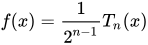
For any given $n\geq 1$ , among the polynomials of degree $n$ with leading coefficient 1 (monic polynomials): $f(x)={\frac {1}{2^{n-1}}}T_{n}(x)$ is the one of which the maximal absolute value on the interval [−1, 1] is minimal.

This maximal absolute value is: ${\frac {1}{2^{n-1}}}$ and $|f(x)|$ reaches this maximum exactly $n+1$ times at: $x=\cos {\frac {k\pi }{n}}\quad {\text{for }}0\leq k\leq n.$

Proof

Let's assume that $w_{n}(x)$ is a polynomial of degree $n$ with leading coefficient 1 with maximal absolute value on the interval [−1, 1] less than 1 / 2^n − 1.

Define $f_{n}(x)={\frac {1}{2^{n-1}}}T_{n}(x)-w_{n}(x)$

Because at extreme points of T_n we have ${\begin{aligned}|w_{n}(x)|&<\left|{\frac {1}{2^{n-1}}}T_{n}(x)\right|\\f_{n}(x)&>0\qquad {\text{ for }}x=\cos {\frac {2k\pi }{n}}&&{\text{ where }}0\leq 2k\leq n\\f_{n}(x)&<0\qquad {\text{ for }}x=\cos {\frac {(2k+1)\pi }{n}}&&{\text{ where }}0\leq 2k+1\leq n\end{aligned}}$

From the intermediate value theorem, f_n(x) has at least n roots. However, this is impossible, as f_n(x) is a polynomial of degree n − 1, so the fundamental theorem of algebra implies it has at most n − 1 roots.

Remark

By the equioscillation theorem, among all the polynomials of degree ≤ n, the polynomial f minimizes ‖ f ‖_∞ on [−1, 1] if and only if there are n + 2 points −1 ≤ x₀ < x₁ < ⋯ < x_{n + 1} ≤ 1 such that | f(x_i)| = ‖ f ‖_∞.

Of course, the null polynomial on the interval [−1, 1] can be approximated by itself and minimizes the ∞-norm.

Above, however, | f | reaches its maximum only n + 1 times because we are searching for the best polynomial of degree n ≥ 1 (therefore the theorem evoked previously cannot be used).

Chebyshev polynomials as special cases of more general polynomial families

The Chebyshev polynomials are a special case of the ultraspherical or Gegenbauer polynomials $C_{n}^{(\lambda )}(x)$ , which themselves are a special case of the Jacobi polynomials $P_{n}^{(\alpha ,\beta )}(x)$ : ${\begin{aligned}T_{n}(x)&={\frac {n}{2}}\lim _{q\to 0}{\frac {1}{q}}C_{n}^{(q)}(x)\qquad {\text{ if }}n\geq 1,\\&={\frac {1}{\binom {n-{\frac {1}{2}}}{n}}}P_{n}^{\left(-{\frac {1}{2}},-{\frac {1}{2}}\right)}(x)={\frac {2^{2n}}{\binom {2n}{n}}}P_{n}^{\left(-{\frac {1}{2}},-{\frac {1}{2}}\right)}(x),\\[2ex]U_{n}(x)&=C_{n}^{(1)}(x)\\&={\frac {n+1}{\binom {n+{\frac {1}{2}}}{n}}}P_{n}^{\left({\frac {1}{2}},{\frac {1}{2}}\right)}(x)={\frac {2^{2n+1}}{\binom {2n+2}{n+1}}}P_{n}^{\left({\frac {1}{2}},{\frac {1}{2}}\right)}(x).\end{aligned}}$

Chebyshev polynomials are also a special case of Dickson polynomials: ${\begin{aligned}D_{n}(2x\alpha ,\alpha ^{2})&=2\alpha ^{n}T_{n}(x),\\E_{n}(2x\alpha ,\alpha ^{2})&=\alpha ^{n}U_{n}(x).\end{aligned}}$ In particular, when $\alpha ={\tfrac {1}{2}}$ , they are related by $D_{n}{\bigl (}x,{\tfrac {1}{4}}{\bigr )}=2^{1-n}T_{n}(x)$ and $E_{n}{\bigl (}x,{\tfrac {1}{4}}{\bigr )}=2^{-n}U_{n}(x)$ .

Other properties

The curves given by y = T_n(x), or equivalently, by the parametric equations y = T_n(cos θ) = cos nθ, x = cos θ, are a special case of Lissajous curves with frequency ratio equal to n.

Similar to the formula: $T_{n}(\cos \theta )=\cos(n\theta ),$ we have the analogous formula: $T_{2n+1}(\sin \theta )={(-1)^{n}\sin }{\bigl (}(2n+1)\theta {\bigr )}.$

For x ≠ 0: $T_{n}\!\left({\frac {x+x^{-1}}{2}}\right)={\frac {x^{n}+x^{-n}}{2}}$ and: $x^{n}=T_{n}\left({\frac {x+x^{-1}}{2}}\right)+{\frac {x-x^{-1}}{2}}U_{n-1}\left({\frac {x+x^{-1}}{2}}\right),$ which follows from the fact that this holds by definition for x = e^iθ.

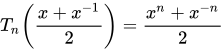
There are relations between Legendre polynomials and Chebyshev polynomials ${\begin{aligned}\sum _{k=0}^{n}P_{k}(x)\,T_{n-k}(x)&=\left(n+1\right)P_{n}(x),\\\sum _{k=0}^{n}P_{k}(x)\,P_{n-k}(x)&=U_{n}(x).\end{aligned}}$ These identities can be proven using generating functions and discrete convolution.

Chebyshev polynomials as determinants

From their definition by recurrence it follows that the Chebyshev polynomials can be obtained as determinants of special tridiagonal matrices of size $k\times k$ :

$T_{k}(x)=\det {\begin{bmatrix}x&1&0&\cdots &0\\1&2x&1&\ddots &\vdots \\0&1&2x&\ddots &0\\\vdots &\ddots &\ddots &\ddots &1\\0&\cdots &0&1&2x\end{bmatrix}},$ and similarly for $U_{k}$ .

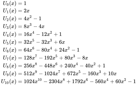
05Examples

First kind

The first few Chebyshev polynomials of the first kind are OEIS: A028297 ${\begin{aligned}T_{0}(x)&=1\\T_{1}(x)&=x\\T_{2}(x)&=2x^{2}-1\\T_{3}(x)&=4x^{3}-3x\\T_{4}(x)&=8x^{4}-8x^{2}+1\\T_{5}(x)&=16x^{5}-20x^{3}+5x\\T_{6}(x)&=32x^{6}-48x^{4}+18x^{2}-1\\T_{7}(x)&=64x^{7}-112x^{5}+56x^{3}-7x\\T_{8}(x)&=128x^{8}-256x^{6}+160x^{4}-32x^{2}+1\\T_{9}(x)&=256x^{9}-576x^{7}+432x^{5}-120x^{3}+9x\\T_{10}(x)&=512x^{10}-1280x^{8}+1120x^{6}-400x^{4}+50x^{2}-1\end{aligned}}$

Second kind

The first few Chebyshev polynomials of the second kind are OEIS: A053117 ${\begin{aligned}U_{0}(x)&=1\\U_{1}(x)&=2x\\U_{2}(x)&=4x^{2}-1\\U_{3}(x)&=8x^{3}-4x\\U_{4}(x)&=16x^{4}-12x^{2}+1\\U_{5}(x)&=32x^{5}-32x^{3}+6x\\U_{6}(x)&=64x^{6}-80x^{4}+24x^{2}-1\\U_{7}(x)&=128x^{7}-192x^{5}+80x^{3}-8x\\U_{8}(x)&=256x^{8}-448x^{6}+240x^{4}-40x^{2}+1\\U_{9}(x)&=512x^{9}-1024x^{7}+672x^{5}-160x^{3}+10x\\U_{10}(x)&=1024x^{10}-2304x^{8}+1792x^{6}-560x^{4}+60x^{2}-1\end{aligned}}$

06As a basis set

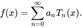
In the appropriate Sobolev space, the set of Chebyshev polynomials form an orthonormal basis, so that a function in the same space can, on −1 ≤ x ≤ 1, be expressed via the expansion: $f(x)=\sum _{n=0}^{\infty }a_{n}T_{n}(x).$ Furthermore, as mentioned previously, the Chebyshev polynomials form an orthogonal basis which (among other things) implies that the coefficients a_n can be determined easily through the application of an inner product. This sum is called a Chebyshev series or a Chebyshev expansion.

Since a Chebyshev series is related to a Fourier cosine series through a change of variables, all of the theorems, identities, etc. that apply to Fourier series have a Chebyshev counterpart. These attributes include:

The Chebyshev polynomials form a complete orthogonal system.
The Chebyshev series converges to f(x) if the function is piecewise smooth and continuous. The smoothness requirement can be relaxed in most cases , as long as there are a finite number of discontinuities in f(x) and its derivatives.
At a discontinuity, the series will converge to the average of the right and left limits.

The abundance of the theorems and identities inherited from Fourier series make the Chebyshev polynomials important tools in numeric analysis; for example they are the most popular general purpose basis functions used in the spectral method, often in favor of trigonometric series due to generally faster convergence for continuous functions (Gibbs' phenomenon is still a problem).

The Chebfun software package supports function manipulation based on their expansion in the Chebyshev basis.

Example 1

Consider the Chebyshev expansion of log(1 + x). One can express: $\log(1+x)=\sum _{n=0}^{\infty }a_{n}T_{n}(x).$

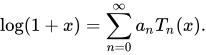
One can find the coefficients a_n either through the application of an inner product or by the discrete orthogonality condition. For the inner product: $\int _{-1}^{+1}{\frac {T_{m}(x)\log(1+x)}{\sqrt {1-x^{2}}}}\,\mathrm {d} x=\sum _{n=0}^{\infty }a_{n}\int _{-1}^{+1}{\frac {T_{m}(x)T_{n}(x)}{\sqrt {1-x^{2}}}}\,\mathrm {d} x,$ which gives: $a_{n}={\begin{cases}-\log 2&{\text{ for }}n=0,\\[3mu]{\dfrac {-2(-1)^{n}}{n}}&{\text{ for }}n>0.\end{cases}}$

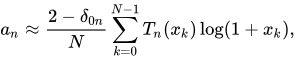
Alternatively, when the inner product of the function being approximated cannot be evaluated, the discrete orthogonality condition gives an often useful result for approximate coefficients: $a_{n}\approx {\frac {2-\delta _{0n}}{N}}\sum _{k=0}^{N-1}T_{n}(x_{k})\log(1+x_{k}),$

where δ_ij is the Kronecker delta function and the x_k are the N Gauss-Chebyshev zeros of T_N(x): $x_{k}=\cos \left({\frac {\pi {\bigl (}k+{\tfrac {1}{2}}{\bigr )}}{N}}\right).$

For any N, these approximate coefficients provide an exact approximation to the function at x_k with a controlled error between those points. The exact coefficients are obtained with N = ∞, thus representing the function exactly at all points in [−1,1]. The rate of convergence depends on the function and its smoothness.

This allows us to compute the approximate coefficients a_n very efficiently through the discrete cosine transform:

$a_{n}\approx {\frac {2-\delta _{0n}}{N}}\sum _{k=0}^{N-1}\cos \left({\frac {n\pi {\bigl (}k+{\tfrac {1}{2}}{\bigr )}}{N}}\right)\log(1+x_{k}).$

Example 2

To provide another example:

${\begin{aligned}\left(1-x^{2}\right)^{\alpha }&=-{\frac {1}{\sqrt {\pi }}}\,{\frac {\Gamma \left({\tfrac {1}{2}}+\alpha \right)}{\Gamma (\alpha +1)}}+2^{1-2\alpha }\,\sum _{n=0}\left(-1\right)^{n}\,{2\alpha \choose \alpha -n}\,T_{2n}(x)\\[1ex]&=2^{-2\alpha }\,\sum _{n=0}\left(-1\right)^{n}\,{2\alpha +1 \choose \alpha -n}\,U_{2n}(x).\end{aligned}}$

Partial sums

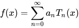
The partial sums of: $f(x)=\sum _{n=0}^{\infty }a_{n}T_{n}(x)$ are very useful in the approximation of various functions and in the solution of differential equations (see spectral method). Two common methods for determining the coefficients a_n are through the use of the inner product as in Galerkin's method and through the use of collocation which is related to interpolation.

As an interpolant, the N coefficients of the (N − 1)st partial sum are usually obtained on the Chebyshev-Gauss-Lobatto points (or Lobatto grid), which results in minimum error and avoids Runge's phenomenon associated with a uniform grid. This collection of points corresponds to the extrema of the highest order polynomial in the sum, plus the endpoints and is given by: $x_{k}=-\cos \left({\frac {k\pi }{N-1}}\right);\qquad k=0,1,\dots ,N-1.$

Polynomial in Chebyshev form

An arbitrary polynomial of degree N can be written in terms of the Chebyshev polynomials of the first kind. Such a polynomial p(x) is of the form: $p(x)=\sum _{n=0}^{N}a_{n}T_{n}(x).$

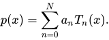
Polynomials in Chebyshev form can be evaluated using the Clenshaw algorithm.

The non-smooth function (top) 3</sup>''H''(−''x'')"}},"i":0}}]}' id="mwAlU">y = −x3H(−x), where H is the Heaviside step function, and (bottom) the 5th partial sum of its Chebyshev expansion. The 7th sum is indistinguishable from the original function at the resolution of the graph.

07Families of polynomials related to Chebyshev polynomials

Polynomials denoted $C_{n}(x)$ and $S_{n}(x)$ closely related to Chebyshev polynomials are sometimes used. They are defined by:

$C_{n}(x)=2T_{n}\left({\frac {x}{2}}\right),\qquad S_{n}(x)=U_{n}\left({\frac {x}{2}}\right)$

and satisfy:

$C_{n}(x)=S_{n}(x)-S_{n-2}(x).$

A. F. Horadam called the polynomials $C_{n}(x)$ Vieta-Lucas polynomials and denoted them $v_{n}(x)$ . He called the polynomials $S_{n}(x)$ Vieta-Fibonacci polynomials and denoted them $V_{n}(x)$ . All of these polynomials have 1 as their leading coefficient. Lists of both sets of polynomials are given in Viète's Opera Mathematica, Chapter IX, Theorems VI and VII. The Vieta-Lucas and Vieta-Fibonacci polynomials of real argument are, up to a power of $i$ and a shift of index in the case of the latter, equal to Lucas and Fibonacci polynomials L_n and F_n of imaginary argument.

Shifted Chebyshev polynomials of the first and second kinds are related to the Chebyshev polynomials by:

${T}_{n}^{*}(x)=T_{n}(2x-1),\qquad {U}_{n}^{*}(x)=U_{n}(2x-1).$

When the argument of the Chebyshev polynomial satisfies 2x − 1 ∈ [−1, 1] the argument of the shifted Chebyshev polynomial satisfies x ∈ [0, 1]. Similarly, one can define shifted polynomials for generic intervals [a, b].

Around 1990 the terms "third-kind" and "fourth-kind" came into use in connection with Chebyshev polynomials, although the polynomials denoted by these terms had an earlier development under the name airfoil polynomials. According to J. C. Mason and G. H. Elliott, the terminology "third-kind" and "fourth-kind" is due to Walter Gautschi, "in consultation with colleagues in the field of orthogonal polynomials." The Chebyshev polynomials of the third kind are defined as:

$V_{n}(x)={\frac {\cos \left(\left(n+{\frac {1}{2}}\right)\theta \right)}{\cos \left({\frac {\theta }{2}}\right)}}={\sqrt {\frac {2}{1+x}}}T_{2n+1}\left({\sqrt {\frac {x+1}{2}}}\right)$ and the Chebyshev polynomials of the fourth kind are defined as: $W_{n}(x)={\frac {\sin \left(\left(n+{\frac {1}{2}}\right)\theta \right)}{{\sin }{\bigl (}{\tfrac {1}{2}}\theta {\bigr )}}}=U_{2n}\left({\sqrt {\frac {x+1}{2}}}\right),$

where $\theta =\arccos x$ . They coincide with the Dirichlet kernel.

In the airfoil literature $V_{n}(x)$ and $W_{n}(x)$ are denoted $t_{n}(x)$ and $u_{n}(x)$ . The polynomial families $T_{n}(x)$ , $U_{n}(x)$ , $V_{n}(x)$ , and $W_{n}(x)$ are orthogonal with respect to the weights: $\left(1-x^{2}\right)^{-1/2},\quad \left(1-x^{2}\right)^{1/2},\quad (1-x)^{-1/2}(1+x)^{1/2},\quad (1+x)^{-1/2}(1-x)^{1/2}$

and are proportional to Jacobi polynomials $P_{n}^{(\alpha ,\beta )}(x)$ with: $(\alpha ,\beta )={\bigl (}{-{\tfrac {1}{2}}},{-{\tfrac {1}{2}}}{\bigr )},\quad (\alpha ,\beta )={\bigl (}{\tfrac {1}{2}},{\tfrac {1}{2}}{\bigr )},\quad (\alpha ,\beta )={\bigl (}{-{\tfrac {1}{2}}},{\tfrac {1}{2}}{\bigr )},\quad (\alpha ,\beta )={\bigl (}{\tfrac {1}{2}},{-{\tfrac {1}{2}}}{\bigr )}.$

All four families satisfy the recurrence $p_{n}(x)=2xp_{n-1}(x)-p_{n-2}(x)$ with $p_{0}(x)=1$ , where $p_{n}=T_{n}$ , $U_{n}$ , $V_{n}$ , or $W_{n}$ , but they differ according to whether $p_{1}(x)$ equals $x$ , $2x$ , $2x-1$ , or $2x+1$ .

Irreducible Factorization of Chebyshev Polynomials

It is easier to discuss this detail by first examining the factorization of the Vieta-Lucas and Vieta-Fibonacci polynomials.

Given the roots of the Chebyshev polynomials, it is easy to see, by comparing their root sets, that $x^{n}C_{n}\left(x+{\frac {1}{x}}\right)=x^{2n}+1$ and $x^{n}S_{n}\left(x+{\frac {1}{x}}\right)=\sum _{k=0}^{n}x^{2k}.$

By expressing the right-hand side expressions in form $x^{2n}+1={\frac {x^{4n}-1}{x^{2n}-1}},$ and $\sum _{k=0}^{n}x^{2k}={\frac {x^{2n+2}-1}{x^{2}-1}},$ the numerators and denominators of these fractions, and consequently the fractions themselves, can be written as products of expressions like $x-g_{i}$ where each $g_{i}$ is a primitive root of unity. Thus, we obtain: $x^{n}C_{n}{\left(x+{\frac {1}{x}}\right)}=\prod _{d\geq 3,\;d\mid 4n,\;d\nmid 2n}\Phi _{d}(x)$ and $x^{n}S_{n}{\left(x+{\frac {1}{x}}\right)}=\prod _{d\geq 3,\;d\mid 2n+2}\Phi _{d}(x),$ where $\Phi _{d}(x)$ is the ⁠ $d$ ⁠th cyclotomic polynomial.

It can be shown that, for every $n\geq 3$ , corresponding to the cyclotomic polynomial $\Phi _{n}(x)$ of degree $\varphi (n)$ there exists a unique polynomial $\Psi _{n}(x)$ of degree $\varphi (n)/2$ such that $x^{\varphi (n)/2}\Psi _{n}{\left(x+{\frac {1}{x}}\right)}=\Phi _{n}(x),$ where $\varphi (n)$ is the well known Euler's totient function.

The polynomials $\Psi _{n}(x)$ may be referred to as cyclotomic pre-polynomials, since the cyclotomic polynomials can be obtained from them via a well-defined mapping.

An obvious property of the mapping $P_{n}(x)\rightarrow x^{n}P_{n}{\left(x+{\frac {1}{x}}\right)}$ applicable to any polynomial $P_{n}(x)$ of degree $n$ is that it maps the product of two or more polynomials to the product of the images of the individual polynomials.

From all of the above, it follows that $C_{n}(x)=\prod _{d\geq 3,\;d\mid 4n,\;d\nmid 2n}\Psi _{d}(x)$ and $S_{n}(x)=\prod _{d\geq 3,\;d\mid 2n+2}\Psi _{d}(x).$

Now, it follows directly that the Chebyshev polynomials $T_{n}(x)$ and $U_{n}(x)$ can be factorized as follows: $T_{n}(x)={\tfrac {1}{2}}\prod _{d\geq 3,\;d\mid 4n,\;d\nmid 2n}\Psi _{d}(2x)$ and $U_{n}(x)=\prod _{d\geq 3,\;d\mid 2n+2}\Psi _{d}(2x).$

From the irreducibility of the polynomials $\Phi _{n}(x)$ it follows that the polynomials $\Psi _{n}(x)$ are also irreducible.

For more details, see .

Even order modified Chebyshev polynomials

Some applications rely on Chebyshev polynomials but may be unable to accommodate the lack of a root at zero, which rules out the use of standard Chebyshev polynomials for these kinds of applications. Even order Chebyshev filter designs using equally terminated passive networks are an example of this. However, even order Chebyshev polynomials may be modified to move the lowest roots down to zero while still maintaining the desirable Chebyshev equi-ripple effect. Such modified polynomials contain two roots at zero, and may be referred to as even order modified Chebyshev polynomials. Even order modified Chebyshev polynomials may be created from the Chebyshev nodes in the same manner as standard Chebyshev polynomials.

$P_{N}=\prod _{i=1}^{N}(x-C_{i})$ where

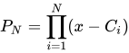
$P_{N}$ is an N-th order Chebyshev polynomial
$C_{i}$ is the i-th Chebyshev node

In the case of even order modified Chebyshev polynomials, the even order modified Chebyshev nodes are used to construct the even order modified Chebyshev polynomials.

$Pe_{N}=\prod _{i=1}^{N}(x-Ce_{i})$ where

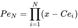
$Pe_{N}$ is an N-th order even order modified Chebyshev polynomial
$Ce_{i}$ is the i-th even order modified Chebyshev node

For example, the 4th order Chebyshev polynomial from the example above is $X^{4}-X^{2}+.125$ , which by inspection contains no roots of zero. Creating the polynomial from the even order modified Chebyshev nodes creates a 4th order even order modified Chebyshev polynomial of $X^{4}-.828427X^{2}$ , which by inspection contains two roots at zero, and may be used in applications requiring roots at zero.

Watch videos about Chebyshev polynomialsExplainers and documentaries on YouTube (opens in a new tab)

Sources and credits

This article is adapted from the Wikipedia article “Chebyshev polynomials”, written by its contributors and licensed under CC BY-SA 4.0. Fathomly has changed the layout, removed citation markers, navigation and maintenance notices, and adjusted punctuation. This adapted version is shared under the same license. For references, see the original article.

Images, from Wikimedia Commons:

Chebyshev Polynomials of the First Kind.svg by Glosser.ca, CC BY-SA 4.0
Chebyshev Polynomials of the Second Kind.svg by Glosser.ca, CC BY-SA 4.0
Chebyshev Polynomials of the 1st Kind (n=0-5, x=(-1,1)).svg by Inductiveload, Public domain
Chebyshev Polynomials of the 2nd Kind (n=0-5, x=(-1,1)).svg by Inductiveload, Public domain
ChebyshevExpansion.png by Ben_pcc (talk) (Uploads), Public domain

Fathomly is not affiliated with or endorsed by the Wikimedia Foundation. Spotted a problem? Tell us.