Encyclopedia

Characteristic function (probability theory)

Fourier transform of the probability density function

Wikipedia contributorsAdapted for Fathomly · View authors

12 min read
Source updated September 4, 2026

In probability theory and statistics, the characteristic function of any real-valued random variable completely defines its probability distribution. If a random variable admits a probability density function, then the characteristic function is the Fourier transform (with sign reversal) of the probability density function. Thus it provides an alternative route to analytical results compared with working directly with probability density functions or cumulative distribution functions. There are particularly simple results for the characteristic functions of distributions defined by the weighted sums of random variables.

In addition to univariate distributions, characteristic functions can be defined for vector- or matrix-valued random variables, and can also be extended to more generic cases.

The characteristic function always exists when treated as a function of a real-valued argument, unlike the moment-generating function. There are relations between the behavior of the characteristic function of a distribution and properties of the distribution, such as the existence of moments and the existence of a density function.

01Introduction

The characteristic function is a way to describe a random variable X. The characteristic function,

$\varphi _{X}(t)=\operatorname {E} \left[e^{itX}\right],$

a function of t, determines the behavior and properties of the probability distribution of X. It is equivalent to a probability density function (if it exists) or cumulative distribution function, in the sense that knowing one of these functions allows computation of the others, but they provide different insights into the features of the random variable.

In particular cases, one or another of these equivalent functions may be easier to represent in terms of simple standard functions.

If a random variable admits a density function, then the characteristic function is its Fourier dual, in the sense that each of them is a Fourier transform of the other. If a random variable has a moment-generating function $M_{X}(t)$ , then the domain of the characteristic function can be extended to the complex plane, and

$\varphi _{X}(-it)=M_{X}(t).$

Note however that the characteristic function of a distribution is well defined for all real values of t, even when the moment-generating function is not well defined for all real values of t.

The characteristic function approach is particularly useful in analysis of linear combinations of independent random variables: a classical proof of the Central Limit Theorem uses characteristic functions and Lévy's continuity theorem. Another important application is to the theory of the decomposability of random variables.

02Definition

Let $X$ be a real-valued random variable. Its characteristic function $\varphi _{X}:\mathbb {R} \to \mathbb {C}$ is defined for each $t\in \mathbb {R}$ as the expected value of $e^{itX}$ , where $i$ is the imaginary unit. $\varphi _{X}(t)=\operatorname {E} \left[e^{itX}\right]=\int _{\mathbb {R} }e^{itx}\,dF_{X}(x)=\int _{0}^{1}e^{itQ_{X}(p)}\,dp=\int _{\mathbb {R} }e^{itx}f_{X}(x)\,dx.$ In the equalites, there is the cumulative distribution function $F_{X}$ , the inverse cumulative distribution function $Q_{X}$ (also called the quantile function), and the density function $f_{X}$ . The integrals are in the Riemann-Stieltjes sense. The last equality holds if $f_{X}$ exists, which then implies that $\varphi _{X}$ is its Fourier transform with sign reversal in the complex exponential. The convention for the constant appearing in the above definition differs from the usual convention for the Fourier transform. For example, some authors define $\varphi _{X}=\left[e^{-2\pi itX}\right]$ , which is essentially a change of parameter. Other notation may be encountered in the literature: ${\hat {p}}$ as the characteristic function for a probability measure $p$ , or ${\hat {f}}$ as the characteristic function corresponding to a density $f$ .

03Generalizations

The notion of characteristic functions generalizes to multivariate random variables and more complicated random elements. The argument of the characteristic function will always belong to the continuous dual of the space where the random variable X takes its values. For common cases such definitions are listed below:

If X is a k-dimensional random vector, then for t ∈ R^k $\varphi _{X}(t)=\operatorname {E} \left[\exp(it^{T}\!X)\right],$ where ${\textstyle t^{T}$ is the transpose of the vector ${\textstyle t$ ,
If X is a k × p-dimensional random matrix, then for t ∈ R^k×p $\varphi _{X}(t)=\operatorname {E} \left[\exp \left(i\operatorname {tr} (t^{T}\!X)\right)\right],$ where ${\textstyle \operatorname {tr} (\cdot )$ is the trace operator,
If X is a complex random variable, then for t ∈ C $\varphi _{X}(t)=\operatorname {E} \left[\exp \left(i\operatorname {Re} \left({\overline {t}}X\right)\right)\right],$ where ${\textstyle {\overline {t}}$ is the complex conjugate of ${\textstyle t$ and ${\textstyle \operatorname {Re} (z)$ is the real part of the complex number ${\textstyle z$ ,
If X is a k-dimensional complex random vector, then for t ∈ C^k $\varphi _{X}(t)=\operatorname {E} \left[\exp(i\operatorname {Re} (t^{*}\!X))\right],$ where ${\textstyle t^{*}$ is the conjugate transpose of the vector ${\textstyle t$ ,
If X(s) is a stochastic process, then for all functions t(s) such that the integral ${\textstyle \int _{\mathbb {R} }t(s)X(s)\,\mathrm {d} s$ converges for almost all realizations of X $\varphi _{X}(t)=\operatorname {E} \left[\exp \left(i\int _{\mathbf {R} }t(s)X(s)\,ds\right)\right].$

04Examples

Distribution	Characteristic function $\varphi (t)$
Degenerate δ_a	$e^{ita}$
Bernoulli Bern(p)	$1-p+pe^{it}$
Binomial B(n, p)	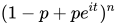$(1-p+pe^{it})^{n}$
Negative binomial NB(r, p)	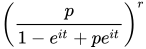$\left({\frac {p}{1-e^{it}+pe^{it}}}\right)^{r}$
Poisson Pois(λ)	$e^{\lambda (e^{it}-1)}$
Uniform (continuous) U(a, b)	${\frac {e^{itb}-e^{ita}}{it(b-a)}}$
Uniform (discrete) DU(a, b)	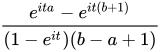${\frac {e^{ita}-e^{it(b+1)}}{(1-e^{it})(b-a+1)}}$
Laplace L(μ, b)	${\frac {e^{it\mu }}{1+b^{2}t^{2}}}$
Logistic Logistic(μ,s)	$e^{i\mu t}{\frac {\pi st}{\sinh(\pi st)}}$
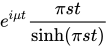Normal N(μ, σ²)	$e^{it\mu -{\frac {1}{2}}\sigma ^{2}t^{2}}$
Chi-squared χ²_k	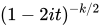$(1-2it)^{-k/2}$
Noncentral chi-squared ${\chi '_{k}}^{2}$	$e^{\frac {i\lambda t}{1-2it}}(1-2it)^{-k/2}$
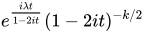Generalized chi-squared ${\tilde {\chi }}({\boldsymbol {w}},{\boldsymbol {k}},{\boldsymbol {\lambda }},s,m)$	${\frac {\exp \left[it\left(m+\sum _{j}{\frac {w_{j}\lambda _{j}}{1-2iw_{j}t}}\right)-{\frac {s^{2}t^{2}}{2}}\right]}{\prod _{j}\left(1-2iw_{j}t\right)^{k_{j}/2}}}$
Cauchy C(μ, θ)	$e^{it\mu -\theta \|t\|}$
Gamma Γ(k, θ)	$(1-it\theta )^{-k}$
Exponential Exp(λ)	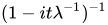$(1-it\lambda ^{-1})^{-1}$
Geometric Gf(p) (number of failures)	${\frac {p}{1-e^{it}(1-p)}}$
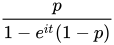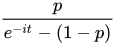
Geometric Gt(p) (number of trials)	${\frac {p}{e^{-it}-(1-p)}}$
Multivariate normal N(μ, Σ)	$e^{i{\mathbf {t} ^{\mathrm {T} }{\boldsymbol {\mu }}}-{\frac {1}{2}}\mathbf {t} ^{\mathrm {T} }{\boldsymbol {\Sigma }}\mathbf {t} }$
Multivariate Cauchy MultiCauchy(μ, Σ)	$e^{i\mathbf {t} ^{\mathrm {T} }{\boldsymbol {\mu }}-{\sqrt {\mathbf {t} ^{\mathrm {T} }{\boldsymbol {\Sigma }}\mathbf {t} }}}$

Oberhettinger (1973) provides extensive tables of characteristic functions.

05Properties

The characteristic function of a real-valued random variable always exists, since it is an integral of a bounded continuous function over a space whose measure is finite.
A characteristic function is uniformly continuous on the entire space.
It is non-vanishing in a region around zero: φ(0) = 1.
It is bounded: |φ(t)| ≤ 1.
It is Hermitian: φ(−t) = φ(t). In particular, the characteristic function of a symmetric (around the origin) random variable is real-valued and even.
There is a bijection between probability distributions and characteristic functions on $\mathbf {R} ^{k}$ , $k\in \mathbb {N}$ . That is, for any two random variables X₁, X₂, with values in $\mathbf {R} ^{k}$ , both have the same probability distribution if and only if $\varphi _{X_{1}}=\varphi _{X_{2}}$ .
If a random variable X has moments up to k-th order, then the characteristic function φ_X is k times continuously differentiable on the entire real line. In this case $\operatorname {E} [X^{k}]=i^{-k}\varphi _{X}^{(k)}(0).$
If a characteristic function φ_X has a k-th derivative at zero, then the random variable X has all moments up to k if k is even, but only up to k, 1 if k is odd. $\varphi _{X}^{(k)}(0)=i^{k}\operatorname {E} [X^{k}]$
If X₁, ..., X_n are independent random variables, and a₁, ..., a_n are some constants, then the characteristic function of the linear combination of the X_i variables is $\varphi _{a_{1}X_{1}+\cdots +a_{n}X_{n}}(t)=\varphi _{X_{1}}(a_{1}t)\cdots \varphi _{X_{n}}(a_{n}t).$ One specific case is the sum of two independent random variables X₁ and X₂ in which case one has $\varphi _{X_{1}+X_{2}}(t)=\varphi _{X_{1}}(t)\cdot \varphi _{X_{2}}(t).$
Let $X$ and $Y$ be two random variables with characteristic functions $\varphi _{X}$ and $\varphi _{Y}$ . $X$ and $Y$ are independent if and only if $\varphi _{X,Y}(s,t)=\varphi _{X}(s)\varphi _{Y}(t)\quad {\text{ for all }}\quad (s,t)\in \mathbb {R} ^{2}$ .
The tail behavior of the characteristic function determines the smoothness of the corresponding density function.
Let the random variable $Y=aX+b$ be the linear transformation of a random variable $X$ . The characteristic function of $Y$ is $\varphi _{Y}(t)=e^{itb}\varphi _{X}(at)$ . For random vectors $X$ and $Y=AX+B$ (where A is a constant matrix and B a constant vector), we have $\varphi _{Y}(t)=e^{it^{\top }B}\varphi _{X}(A^{\top }t)$ .

Continuity

The bijection stated above between probability distributions and characteristic functions is sequentially continuous. That is, whenever a sequence of distribution functions F_j(x) converges (weakly) to some distribution F(x), the corresponding sequence of characteristic functions φ_j(t) will also converge, and the limit φ(t) will correspond to the characteristic function of law F. More formally, this is stated as

Lévy’s continuity theorem: A sequence X_j of n-variate random variables converges in distribution to random variable X if and only if the sequence φ_{X_j} converges pointwise to a function φ which is continuous at the origin. Where φ is the characteristic function of X.

This theorem can be used to prove the law of large numbers and the central limit theorem.

Inversion formula

There is a one-to-one correspondence between cumulative distribution functions and characteristic functions, so it is possible to find one of these functions if we know the other. The formula in the definition of characteristic function allows us to compute φ when we know the distribution function F (or density f). If, on the other hand, we know the characteristic function φ and want to find the corresponding distribution function, then one of the following inversion theorems can be used.

Theorem. If the characteristic function φ_X of a random variable X is integrable, then F_X is absolutely continuous, and therefore X has a probability density function. In the univariate case (i.e. when X is scalar-valued) the density function is given by $f_{X}(x)=F_{X}'(x)={\frac {1}{2\pi }}\int _{\mathbf {R} }e^{-itx}\varphi _{X}(t)\,dt.$

In the multivariate case it is $f_{X}(x)={\frac {1}{(2\pi )^{n}}}\int _{\mathbf {R} ^{n}}e^{-i(t\cdot x)}\varphi _{X}(t)\lambda (dt)$

where ${\textstyle t\cdot x$ is the dot product.

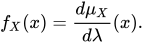
The density function is the Radon-Nikodym derivative of the distribution μ_X with respect to the Lebesgue measure λ: $f_{X}(x)={\frac {d\mu _{X}}{d\lambda }}(x).$

Theorem (Lévy). If φ_X is characteristic function of distribution function F_X, two points a < b are such that {x | a < x < b} is a continuity set of μ_X (in the univariate case this condition is equivalent to continuity of F_X at points a and b), then

If X is scalar: $F_{X}(b)-F_{X}(a)={\frac {1}{2\pi }}\lim _{T\to \infty }\int _{-T}^{+T}{\frac {e^{-ita}-e^{-itb}}{it}}\,\varphi _{X}(t)\,dt.$ This formula can be re-stated in a form more convenient for numerical computation as ${\frac {F(x+h)-F(x-h)}{2h}}={\frac {1}{2\pi }}\int _{-\infty }^{\infty }{\frac {\sin ht}{ht}}e^{-itx}\varphi _{X}(t)\,dt.$ For a random variable bounded from below one can obtain $F(b)$ by taking $a$ such that $F(a)=0.$ Otherwise, if a random variable is not bounded from below, the limit for $a\to -\infty$ gives $F(b)$ , but is numerically impractical.
If X is a vector random variable: $\mu _{X}{\big (}\{a<x<b\}{\big )}={\frac {1}{(2\pi )^{n}}}\lim _{T_{1}\to \infty }\cdots \lim _{T_{n}\to \infty }\int \limits _{-T_{1}\leq t_{1}\leq T_{1}}\cdots \int \limits _{-T_{n}\leq t_{n}\leq T_{n}}\prod _{k=1}^{n}\left({\frac {e^{-it_{k}a_{k}}-e^{-it_{k}b_{k}}}{it_{k}}}\right)\varphi _{X}(t)\lambda (dt_{1}\times \cdots \times dt_{n})$

Theorem. If a is (possibly) an atom of X (in the univariate case this means a point of discontinuity of F_X) then

If X is scalar: $F_{X}(a)-F_{X}(a-0)=\lim _{T\to \infty }{\frac {1}{2T}}\int _{-T}^{+T}e^{-ita}\varphi _{X}(t)\,dt$
If X is a vector random variable: $\mu _{X}(\{a\})=\lim _{T_{1}\to \infty }\cdots \lim _{T_{n}\to \infty }\left(\prod _{k=1}^{n}{\frac {1}{2T_{k}}}\right)\int \limits _{[-T_{1},T_{1}]\times \dots \times [-T_{n},T_{n}]}e^{-i(t\cdot a)}\varphi _{X}(t)\lambda (dt)$

Theorem (Gil-Pelaez). For a univariate random variable X, if x is a continuity point of F_X then

$F_{X}(x)={\frac {1}{2}}-{\frac {1}{\pi }}\int _{0}^{\infty }{\frac {\operatorname {Im} [e^{-itx}\varphi _{X}(t)]}{t}}\,dt$

where the imaginary part of a complex number $z$ is given by $\mathrm {Im} (z)=(z-z^{*})/2i$ .

And its density function is:

$f_{X}(x)={\frac {1}{\pi }}\int _{0}^{\infty }\operatorname {Re} [e^{-itx}\varphi _{X}(t)]\,dt$

The integral may be not Lebesgue-integrable; for example, when X is the discrete random variable that is always 0, it becomes the Dirichlet integral.

Inversion formulas for multivariate distributions are available.

Criteria for characteristic functions

The set of all characteristic functions is closed under certain operations:

A convex linear combination ${\textstyle \sum _{n}a_{n}\varphi _{n}(t)$ (with ${\textstyle a_{n}\geq 0,\ \sum _{n}a_{n}=1$ ) of a finite or a countable number of characteristic functions is also a characteristic function.
The product of a finite number of characteristic functions is also a characteristic function. The same holds for an infinite product provided that it converges to a function continuous at the origin.
If φ is a characteristic function and α is a real number, then ${\bar {\varphi }}$ , Re(φ), |φ|², and φ(αt) are also characteristic functions.

It is well known that any non-decreasing càdlàg function F with limits F(−∞) = 0, F(+∞) = 1 corresponds to a cumulative distribution function of some random variable. There is also interest in finding similar simple criteria for when a given function φ could be the characteristic function of some random variable. The central result here is Bochner’s theorem, although its usefulness is limited because the main condition of the theorem, non-negative definiteness, is very hard to verify. Other theorems also exist, such as Khinchine’s, Mathias’s, or Cramér’s, although their application is just as difficult. Pólya’s theorem, on the other hand, provides a very simple convexity condition which is sufficient but not necessary. Characteristic functions which satisfy this condition are called Pólya-type.

Bochner’s theorem. An arbitrary function φ : Rⁿ → C is the characteristic function of some random variable if and only if φ is positive definite, continuous at the origin, and if φ(0) = 1.

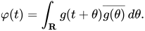
Khinchine’s criterion. A complex-valued, absolutely continuous function φ, with φ(0) = 1, is a characteristic function if and only if it admits the representation

$\varphi (t)=\int _{\mathbf {R} }g(t+\theta ){\overline {g(\theta )}}\,d\theta .$

Mathias’ theorem. A real-valued, even, continuous, absolutely integrable function φ, with φ(0) = 1, is a characteristic function if and only if

$(-1)^{n}\left(\int _{\mathbf {R} }\varphi (pt)e^{-t^{2}/2}H_{2n}(t)\,dt\right)\geq 0$

for n = 0,1,2,..., and all p > 0. Here H_2n denotes the Hermite polynomial of degree 2n.

Pólya’s theorem. If $\varphi$ is a real-valued, even, continuous function which satisfies the conditions

$\varphi (0)=1$ ,
$\varphi$ is convex for $t>0$ ,
$\varphi (\infty )=0$ ,

then φ(t) is the characteristic function of an absolutely continuous distribution symmetric about 0.

06Uses

Because of the continuity theorem, characteristic functions are used in the most frequently seen proof of the central limit theorem. The main technique involved in making calculations with a characteristic function is recognizing the function as the characteristic function of a particular distribution.

Basic manipulations of distributions

Characteristic functions are particularly useful for dealing with linear functions of independent random variables. For example, if X₁, X₂, ..., X_n is a sequence of independent (and not necessarily identically distributed) random variables, and

$S_{n}=\sum _{i=1}^{n}a_{i}X_{i},\,\!$

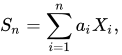
where the a_i are constants, then the characteristic function for S_n is given by

$\varphi _{S_{n}}(t)=\varphi _{X_{1}}(a_{1}t)\varphi _{X_{2}}(a_{2}t)\cdots \varphi _{X_{n}}(a_{n}t)\,\!$

In particular, φ_X+Y(t) = φ_X(t)φ_Y(t). To see this, write out the definition of characteristic function:

$\varphi _{X+Y}(t)=\operatorname {E} \left[e^{it(X+Y)}\right]=\operatorname {E} \left[e^{itX}e^{itY}\right]=\operatorname {E} \left[e^{itX}\right]\operatorname {E} \left[e^{itY}\right]=\varphi _{X}(t)\varphi _{Y}(t)$

The independence of X and Y is required to establish the equality of the third and fourth expressions.

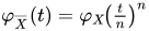
Another special case of interest for identically distributed random variables is when a_i = 1 / n and then S_n is the sample mean. In this case, writing X for the mean,

$\varphi _{\overline {X}}(t)=\varphi _{X}\!\left({\tfrac {t}{n}}\right)^{n}$

Moments

Characteristic functions can also be used to find moments of a random variable. Provided that the n-^th moment exists, the characteristic function can be differentiated n times:

$\operatorname {E} \left[X^{n}\right]=i^{-n}\left[{\frac {d^{n}}{dt^{n}}}\varphi _{X}(t)\right]_{t=0}=i^{-n}\varphi _{X}^{(n)}(0),\!$

This can be formally written using the derivatives of the Dirac delta function: $f_{X}(x)=\sum _{n=0}^{\infty }{\frac {(-1)^{n}}{n!}}\delta ^{(n)}(x)\operatorname {E} [X^{n}]$ which allows a formal solution to the moment problem. For example, suppose X has a standard Cauchy distribution. Then φ_X(t) = e^−|t|. This is not differentiable at t = 0, showing that the Cauchy distribution has no expectation. Also, the characteristic function of the sample mean X of n independent observations has characteristic function φ_X(t) = (e^−|t|/n)ⁿ = e^−|t|, using the result from the previous section. This is the characteristic function of the standard Cauchy distribution: thus, the sample mean has the same distribution as the population itself.

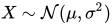
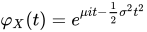
As a further example, suppose X follows a Gaussian distribution i.e. $X\sim {\mathcal {N}}(\mu ,\sigma ^{2})$ . Then $\varphi _{X}(t)=e^{\mu it-{\frac {1}{2}}\sigma ^{2}t^{2}}$ and

$\operatorname {E} \left[X\right]=i^{-1}\left[{\frac {d}{dt}}\varphi _{X}(t)\right]_{t=0}=i^{-1}\left[(i\mu -\sigma ^{2}t)\varphi _{X}(t)\right]_{t=0}=\mu$

A similar calculation shows $\operatorname {E} \left[X^{2}\right]=\mu ^{2}+\sigma ^{2}$ and is easier to carry out than applying the definition of expectation and using integration by parts to evaluate $\operatorname {E} \left[X^{2}\right]$ .

The logarithm of a characteristic function is a cumulant generating function, which is useful for finding cumulants; some instead define the cumulant generating function as the logarithm of the moment-generating function, and call the logarithm of the characteristic function the second cumulant generating function.

Data analysis

Characteristic functions can be used as part of procedures for fitting probability distributions to samples of data. Cases where this provides a practicable option compared to other possibilities include fitting the stable distribution since closed form expressions for the density are not available which makes implementation of maximum likelihood estimation difficult. Estimation procedures are available which match the theoretical characteristic function to the empirical characteristic function, calculated from the data. Paulson et al. (1975) and Heathcote (1977) provide some theoretical background for such an estimation procedure. In addition, Yu (2004) describes applications of empirical characteristic functions to fit time series models where likelihood procedures are impractical. Empirical characteristic functions have also been used by Ansari et al. (2020) and Li et al. (2020) for training generative adversarial networks.

Example

The gamma distribution with scale parameter θ and a shape parameter k has the characteristic function

$(1-\theta it)^{-k}.$

Now suppose that we have

$X~\sim \Gamma (k_{1},\theta ){\mbox{ and }}Y\sim \Gamma (k_{2},\theta )$

with X and Y independent from each other, and we wish to know what the distribution of X + Y is. The characteristic functions are

$\varphi _{X}(t)=(1-\theta it)^{-k_{1}},\,\qquad \varphi _{Y}(t)=(1-\theta it)^{-k_{2}}$

which by independence and the basic properties of characteristic function leads to

$\varphi _{X+Y}(t)=\varphi _{X}(t)\varphi _{Y}(t)=(1-\theta it)^{-k_{1}}(1-\theta it)^{-k_{2}}=\left(1-\theta it\right)^{-(k_{1}+k_{2})}.$

This is the characteristic function of the gamma distribution scale parameter θ and shape parameter k₁ + k₂, and we therefore conclude

$X+Y\sim \Gamma (k_{1}+k_{2},\theta )$

The result can be expanded to n independent gamma distributed random variables with the same scale parameter and we get

$\forall i\in \{1,\ldots ,n\}:X_{i}\sim \Gamma (k_{i},\theta )\qquad \Rightarrow \qquad \sum _{i=1}^{n}X_{i}\sim \Gamma \left(\sum _{i=1}^{n}k_{i},\theta \right).$

07Entire characteristic functions

As defined above, the argument of the characteristic function is treated as a real number: however, certain aspects of the theory of characteristic functions are advanced by extending the definition into the complex plane by analytic continuation, in cases where this is possible.

08Characteristic function of a random variable with values in a locally compact Abelian group

Let $X$ be a locally compact Abelian group, let $Y$ be its character group, and let $(x,y)$ the value of a character $y\in Y$ at an element $x\in X$ . Let $\xi$ be a random variable with values in $X$ , and let $\mu$ be its distribution. The characteristic function of the random variable $\xi$ (distribution $\mu$ ) is defined by

$\mathbf {E} [(\xi ,y)]={\widehat {\mu }}(y)=\int _{X}(x,y)\,d\mu (x),\quad y\in Y.$

Watch videos about Characteristic function (probability theory)Explainers and documentaries on YouTube (opens in a new tab)

Sources and credits

This article is adapted from the Wikipedia article “Characteristic function (probability theory)”, written by its contributors and licensed under CC BY-SA 4.0. Fathomly has changed the layout, removed citation markers, navigation and maintenance notices, and adjusted punctuation. This adapted version is shared under the same license. For references, see the original article.

Images, from Wikimedia Commons:

Sinc simple.svg by Stpasha, Public domain
2 cfs coincide over a finite interval.svg by Stpasha, Public domain

Fathomly is not affiliated with or endorsed by the Wikimedia Foundation. Spotted a problem? Tell us.

Characteristic function (probability theory)

01Introduction

02Definition

03Generalizations

04Examples