Moment generating function
Concept in probability theory and statistics
In probability theory and statistics, the moment generating function of a real-valued random variable is a generating function that provides an alternative specification of the random variable's probability distribution. Thus, it provides the basis of an alternative route to analytical results compared with working directly with probability density functions or cumulative distribution functions. There are particularly simple results for the moment generating functions of distributions defined by the weighted sums of random variables. However, not all random variables have moment generating functions.
As its name implies, the moment generating function can be used to compute a distribution’s moments: the n-th moment about 0 is the n-th derivative of the moment generating function, evaluated at 0.
In addition to univariate real-valued distributions, moment generating functions can also be defined for vector- or matrix-valued random variables, and can even be extended to more general cases.
The moment generating function of a real-valued distribution does not always exist, unlike the characteristic function. There are relations between the behavior of the moment generating function of a distribution and properties of the distribution, such as the existence of moments.
01Definition
Let 


![M_{X}(t)=\operatorname {E} \left[e^{tX}\right]](https://wikimedia.org/api/rest_v1/media/math/render/svg/bbdb8d436c1f3850882f911bf91695539de698e6)
provided this expectation exists for 


![\operatorname {E} \left[e^{tX}\right]](https://wikimedia.org/api/rest_v1/media/math/render/svg/ad12410185c69f6ffc6889791e227412a323406d)
In other words, the moment generating function of X is the expectation of the random variable 



![M_{\mathbf {X} }(\mathbf {t} ):=\operatorname {E} \left[e^{\mathbf {t} ^{\mathrm {T} }\mathbf {X} }\right].](https://wikimedia.org/api/rest_v1/media/math/render/svg/c011b36227dfd4b8347c2d863f9d8d9ea86391da)

The moment generating function is so named because it can be used to find the moments of the distribution. The series expansion of

Hence,
![{\begin{aligned}M_{X}(t)&=\operatorname {E} [e^{tX}]\\[1ex]&=1+t\operatorname {E} [X]+{\frac {t^{2}\operatorname {E} [X^{2}]}{2!}}+{\frac {t^{3}\operatorname {E} [X^{3}]}{3!}}+\cdots +{\frac {t^{n}\operatorname {E} [X^{n}]}{n!}}+\cdots \\[1ex]&=1+tm_{1}+{\frac {t^{2}m_{2}}{2!}}+{\frac {t^{3}m_{3}}{3!}}+\cdots +{\frac {t^{n}m_{n}}{n!}}+\cdots ,\end{aligned}}](https://wikimedia.org/api/rest_v1/media/math/render/svg/3fa03289678b5e409ea1928a971dc7f64bcedfed)
where 


If 

since the PDF's two-sided Laplace transform is given as

and the moment generating function's definition expands (by the law of the unconscious statistician) to
![M_{X}(t)=\operatorname {E} \left[e^{tX}\right]=\int _{-\infty }^{\infty }e^{tx}f_{X}(x)\,dx.](https://wikimedia.org/api/rest_v1/media/math/render/svg/9300f3511ab8b775f02ea222c7d2dd631c7cded5)
This is consistent with the characteristic function of 

02Examples
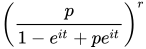
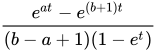
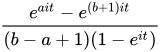
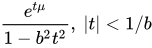
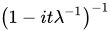
Here are some examples of the moment generating function and the characteristic function for comparison. It can be seen that the characteristic function is a Wick rotation of the moment generating function
| Distribution | moment generating function |
Characteristic function  |
|---|---|---|
Degenerate  |
 |
 |
Bernoulli 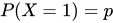 |
 |
 |
Binomial  |
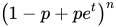 |
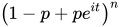 |
Geometric  |
 |
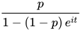 |
Negative binomial  |
 |
 |
Poisson  |
 |
 |
Uniform (continuous)  |
 |
 |
Uniform (discrete)  |
 |
 |
Laplace  |
 |
 |
Normal  |
 |
 |
Chi-squared  |
 |
 |
Noncentral chi-squared  |
 |
 |
Gamma  |
 |
 |
Exponential  |
 |
 |
| Beta | 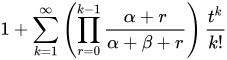 |
 (see Confluent hypergeometric function) |
Multivariate normal  |
![\exp \left[\mathbf {t} ^{\mathrm {T} }\left({\boldsymbol {\mu }}+{\tfrac {1}{2}}{\boldsymbol {\Sigma }}\mathbf {t} \right)\right]](https://wikimedia.org/api/rest_v1/media/math/render/svg/12c98412167dac079ac9f2d0ec5c362148b1a2a3) |
![\exp \left[\mathbf {t} ^{\mathrm {T} }\left(i{\boldsymbol {\mu }}-{\tfrac {1}{2}}{\boldsymbol {\Sigma }}\mathbf {t} \right)\right]](https://wikimedia.org/api/rest_v1/media/math/render/svg/1e70a6b9df258b2dfb1fc7bbfdd5ae81d8df9774) |
Cauchy 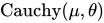 |
Does not exist |  |
| Multivariate Cauchy
|
Does not exist |  |

03Calculation
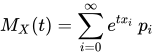
The moment generating function is the expectation of a function of the random variable, it can be written as:
- For a discrete probability mass function,
- For a continuous probability density function,
- In the general case:
, using the Riemann-Stieltjes integral, and where
is the cumulative distribution function. This is simply the Laplace-Stieltjes transform of
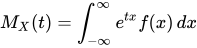
Note that for the case where 
![{\begin{aligned}M_{X}(t)&=\int _{-\infty }^{\infty }e^{tx}f(x)\,dx\\[1ex]&=\int _{-\infty }^{\infty }\left(1+tx+{\frac {t^{2}x^{2}}{2!}}+\cdots +{\frac {t^{n}x^{n}}{n!}}+\cdots \right)f(x)\,dx\\[1ex]&=1+tm_{1}+{\frac {t^{2}m_{2}}{2!}}+\cdots +{\frac {t^{n}m_{n}}{n!}}+\cdots ,\end{aligned}}](https://wikimedia.org/api/rest_v1/media/math/render/svg/9a53864070a933cc8c458ccdb73e74be29be2574)
where
Linear transformations of random variables
If random variable 

![M_{\alpha X+\beta }(t)=\operatorname {E} \left[e^{(\alpha X+\beta )t}\right]=e^{\beta t}\operatorname {E} \left[e^{\alpha Xt}\right]=e^{\beta t}M_{X}(\alpha t)](https://wikimedia.org/api/rest_v1/media/math/render/svg/b5f8720a8a3a0499893b524bf86e45024a60edde)
Linear combination of independent random variables
If 

Vector-valued random variables
For vector-valued random variables 
![M_{X}(\mathbf {t} )=\operatorname {E} \left[e^{\langle \mathbf {t} ,\mathbf {X} \rangle }\right]](https://wikimedia.org/api/rest_v1/media/math/render/svg/db58e19def5c9327516aeec91f1d505c307015cb)
where 
04Important properties
Moment generating functions are positive and log-convex, with M(0) = 1.
An important property of the moment generating function is that it uniquely determines the distribution. In other words, if 


for all values of x (or equivalently X and Y have the same distribution). This statement is not equivalent to the statement "if two distributions have the same moments, then they are identical at all points." This is because in some cases, the moments exist and yet the moment generating function does not, because the limit

may not exist. The log-normal distribution is an example of when this occurs: its moments are ![\operatorname {E} [X^{n}]=e^{n\mu +n^{2}\sigma ^{2}/2}](https://wikimedia.org/api/rest_v1/media/math/render/svg/1ec49bbb5852b6e735f0a6a49468771db326b7bf)
Calculations of moments
The moment generating function is so called because if it exists on an open interval around t = 0, then it is the exponential generating function of the moments of the probability distribution:
![m_{n}=\operatorname {E} \left[X^{n}\right]=M_{X}^{(n)}(0)=\left.{\frac {d^{n}M_{X}}{dt^{n}}}\right|_{t=0}.](https://wikimedia.org/api/rest_v1/media/math/render/svg/75c325a464230f75e64dbdfed1c349b10d20a667)
That is, with n being a nonnegative integer, the n-th moment about 0 is the n-th derivative of the moment generating function, evaluated at t = 0.
05Other properties
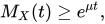
Jensen's inequality provides a simple lower bound on the moment generating function:

The moment generating function can be used in conjunction with Markov's inequality to bound the upper tail of a real random variable X. This statement is also called the Chernoff bound. Since 

![\Pr(X\geq a)=\Pr(e^{tX}\geq e^{ta})\leq e^{-at}\operatorname {E} \left[e^{tX}\right]=e^{-at}M_{X}(t)](https://wikimedia.org/api/rest_v1/media/math/render/svg/fe4cc57423e745b2fda5a1bdba8209a7cfe60ed5)


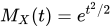

Various lemmas, such as Hoeffding's lemma or Bennett's inequality provide bounds on the moment generating function in the case of a zero-mean, bounded random variable.
When ![\operatorname {E} [X^{m}]\leq \left({\frac {m}{te}}\right)^{m}M_{X}(t),](https://wikimedia.org/api/rest_v1/media/math/render/svg/6e87f3682520c940b04777b9ede4a583ab6a761a)

This follows from the inequality 
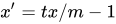
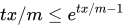



![\operatorname {E} [X^{m}]](https://wikimedia.org/api/rest_v1/media/math/render/svg/7d31d9b6f4e262bfe8a57810801515535c37f270)
![\operatorname {E} [e^{tX}]](https://wikimedia.org/api/rest_v1/media/math/render/svg/0379eb85a8f71d1d2e06107ba42758bc26c355b6)
As an example, consider 



![\operatorname {E} [X^{m}]\leq {\left(1+2m/k\right)}^{k/2}e^{-m}{\left(k+2m\right)}^{m}.](https://wikimedia.org/api/rest_v1/media/math/render/svg/2ff539fd3271a9a74a9e224c3ff8fbc4cf0d51dc)
![\operatorname {E} [X^{m}]\leq 2^{m}\Gamma (m+k/2)/\Gamma (k/2)](https://wikimedia.org/api/rest_v1/media/math/render/svg/49b3e93bf6b119412e575abc6a3af7744b11d2da)


06Relation to other functions
Related to the moment generating function are a number of other transforms that are common in probability theory:
- Characteristic function
- The characteristic function
is related to the moment generating function via
the characteristic function is the moment generating function of iX or the moment generating function of X evaluated on the imaginary axis. This function can also be viewed as the Fourier transform of the probability density function, which can therefore be deduced from it by inverse Fourier transform.
- Cumulant-generating function
- The cumulant-generating function is defined as the logarithm of the moment generating function; some instead define the cumulant-generating function as the logarithm of the characteristic function, while others call this latter the second cumulant-generating function.
- Probability-generating function
- The probability-generating function is defined as
This immediately implies that
![G(e^{t})=\operatorname {E} \left[e^{tX}\right]=M_{X}(t).](https://wikimedia.org/api/rest_v1/media/math/render/svg/ec22810d622164a684da4b6f970dd0dbd1dbeac4)
Sources and credits
This article is adapted from the Wikipedia article “Moment generating function”, written by its contributors and licensed under CC BY-SA 4.0. Fathomly has changed the layout, removed citation markers, navigation and maintenance notices, and adjusted punctuation. This adapted version is shared under the same license. For references, see the original article.
Fathomly is not affiliated with or endorsed by the Wikimedia Foundation. Spotted a problem? Tell us.
