Activation function
Artificial neural network node function

In artificial neural networks, the activation function of a node is a function that calculates the output of the node based on its individual inputs and their weights. Nontrivial problems can be solved using only a few nodes if the activation function is nonlinear.
Modern activation functions include the logistic (sigmoid) function used in the 2012 speech recognition model developed by Hinton et al; the ReLU used in the 2012 AlexNet computer vision model and in the 2015 ResNet model; and the smooth version of the ReLU, the GELU, which was used in the 2018 BERT model.
01Comparison of activation functions
Aside from their empirical performance, activation functions also have different mathematical properties:
- Nonlinear
- When the activation function is non-linear, then a two-layer neural network can be proven to be a universal function approximator. This is known as the Universal Approximation Theorem. The identity activation function does not satisfy this property. When multiple layers use the identity activation function, the entire network is equivalent to a single-layer model.
- Range
- When the range of the activation function is finite, gradient-based training methods tend to be more stable, because pattern presentations significantly affect only limited weights. When the range is infinite, training is generally more efficient because pattern presentations significantly affect most of the weights. In the latter case, smaller learning rates are typically necessary.
- Continuously differentiable
- This property is desirable for enabling gradient-based optimization methods (ReLU is not continuously differentiable and has some issues with gradient-based optimization, but it is still possible). The binary step activation function is not differentiable at 0, and it differentiates to 0 for all other values, so gradient-based methods can make no progress with it.
These properties do not decisively influence performance, nor are they the only mathematical properties that may be useful. For instance, the strictly positive range of the softplus makes it suitable for predicting variances in variational autoencoders.

02Mathematical details
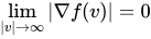
The most common activation functions can be divided into three categories: ridge functions, radial functions and fold functions.
An activation function 

Ridge activation functions
Ridge functions are multivariate functions acting on a linear combination of the input variables. Often used examples include:
 ,
, ,
, .
.In biologically inspired neural networks, the activation function is usually an abstraction representing the rate of action potential firing in the cell. In its simplest form, this function is binary, that is, either the neuron is firing or not.
Neurons also cannot fire faster than a certain rate. This biological limitation motivates the use of sigmoid activation functions, whose output range is confined to a finite interval.
The function looks like 

If a line has a positive slope, on the other hand, it may reflect the increase in firing rate that occurs as input current increases. Such a function would be of the form 
Radial activation functions
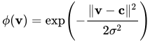
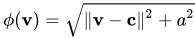
A special class of activation functions known as radial basis functions (RBFs) are used in RBF networks. These activation functions can take many forms, but they are usually found as one of the following functions:
- Gaussian:
- Multiquadratics:
- Inverse multiquadratics:
- Polyharmonic splines

where 


Other examples
Periodic functions can serve as activation functions. Usually the sinusoid is used, as any periodic function is decomposable into sinusoids by the Fourier transform.
Quadratic activation maps 
Folding activation functions
Folding activation functions are extensively used in the pooling layers in convolutional neural networks, and in output layers of multiclass classification networks. These activations perform aggregation over the inputs, such as taking the mean, minimum or maximum. In multiclass classification the softmax activation is often used.
Table of activation functions
The following table compares the properties of several activation functions that are functions of one fold x from the previous layer or layers:
| Name | Plot | Function,  |
Derivative of  , ,  |
Range | Order of continuity |
|---|---|---|---|---|---|
| Identity |  |
 |
 |
 | |
| Binary step | 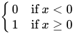 |
 |
 |
 | |
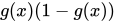
| Logistic, sigmoid, or soft step | 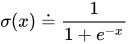 |
 |
 |
| |
| Hyperbolic tangent (tanh) | 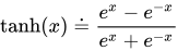 |
 |
 |
| |
| Soboleva modified hyperbolic tangent (smht) | 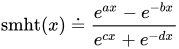 |
|
| ||
| Softsign |  |
 |
|
 | |
| Rectified linear unit (ReLU) | 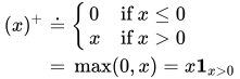 |
 |
 |
 | |
| Gaussian Error Linear Unit (GELU) | 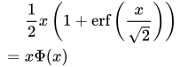 where where  is the gaussian error function. is the gaussian error function. |
 where where 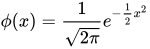 is the probability density function of standard gaussian distribution. is the probability density function of standard gaussian distribution. |
 |
| |
| Softplus |  |
 |
 |
| |
| Exponential linear unit (ELU) | 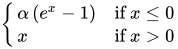
|
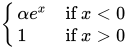 |
 |
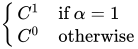 | |
| Scaled exponential linear unit (SELU) | 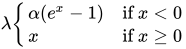
|
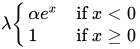 |
 |
| |
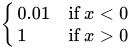
| Leaky rectified linear unit (Leaky ReLU) | 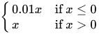 |
 |
|
| |
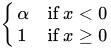
| Parametric rectified linear unit (PReLU) | 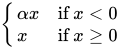
|
 |
|
| |
| Rectified Parametric Sigmoid Units (flexible, 5 parameters) | 
where
|
 |
|
| |
| Sigmoid linear unit (SiLU, Sigmoid shrinkage, SiL, or Swish-1) |  |
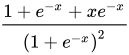 |
 |
| |
| Exponential Linear Sigmoid SquasHing (ELiSH) |  |
 |
 |
| |
| Gaussian |  |
 |
![(0,1]](https://wikimedia.org/api/rest_v1/media/math/render/svg/7e70f9c241f9faa8e9fdda2e8b238e288807d7a4) |
| |
| Sinusoid |  |
 |
![[-1,1]](https://wikimedia.org/api/rest_v1/media/math/render/svg/51e3b7f14a6f70e614728c583409a0b9a8b9de01) |
|

 and
and 

The following table lists activation functions that are not functions of a single fold x from the previous layer or layers:
| Name | Equation,  |
Derivatives,  |
Range | Order of continuity |
|---|---|---|---|---|
| Softmax |  for i = 1, ..., J for i = 1, ..., J |
 |
|
|
| Maxout |  |
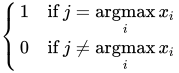 |
|
|
- ^ Here,
is the Kronecker delta.
- ^ For instance,
could be iterating through the number of kernels of the previous neural network layer while
iterates through the number of kernels of the current layer.
Quantum activation functions
In quantum neural networks programmed on gate-model quantum computers, based on quantum perceptrons instead of variational quantum circuits, the non-linearity of the activation function can be implemented with no need of measuring the output of each perceptron at each layer. The quantum properties loaded within the circuit such as superposition can be preserved by creating the Taylor series of the argument computed by the perceptron itself, with suitable quantum circuits computing the powers up to a wanted approximation degree. Because of the flexibility of such quantum circuits, they can be designed in order to approximate any arbitrary classical activation function.
Sources and credits
This article is adapted from the Wikipedia article “Activation function”, written by its contributors and licensed under CC BY-SA 4.0. Fathomly has changed the layout, removed citation markers, navigation and maintenance notices, and adjusted punctuation. This adapted version is shared under the same license. For references, see the original article.
Images, from Wikimedia Commons:
- Logistic-curve.svg by Qef (talk), Public domain
- ReLU and GELU.svg by Ringdongdang, CC BY-SA 4.0
Fathomly is not affiliated with or endorsed by the Wikimedia Foundation. Spotted a problem? Tell us.
