Encyclopedia

Radial basis function

Type of mathematical function

Wikipedia contributorsAdapted for Fathomly · View authors

4 min read
Source updated October 29, 2025

In mathematics a radial basis function (RBF) is a real-valued function ${\textstyle \varphi$ whose value depends only on the distance between the input and some fixed point, either the origin, so that ${\textstyle \varphi (\mathbf {x} )={\hat {\varphi }}(\left\|\mathbf {x} \right\|)$ , or some other fixed point ${\textstyle \mathbf {c}$ , called a center, so that ${\textstyle \varphi (\mathbf {x} )={\hat {\varphi }}(\left\|\mathbf {x} -\mathbf {c} \right\|)$ . Any function ${\textstyle \varphi$ that satisfies the property ${\textstyle \varphi (\mathbf {x} )={\hat {\varphi }}(\left\|\mathbf {x} \right\|)$ is a radial function. The distance is usually Euclidean distance, although other metrics are sometimes used. They are often used as a collection $\{\varphi _{k}\}_{k}$ which forms a basis for some function space of interest, hence the name.

Sums of radial basis functions are typically used to approximate given functions. This approximation process can also be interpreted as a simple kind of neural network; this was the context in which they were originally applied to machine learning, in work by David Broomhead and David Lowe in 1988, which stemmed from Michael J. D. Powell's seminal research from 1977. RBFs are also used as a kernel in support vector classification. The technique has proven effective and flexible enough that radial basis functions are now applied in a variety of engineering applications.

01Definition

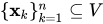
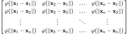
A radial function is a function ${\textstyle \varphi :[0,\infty )\to \mathbb {R}$ . When paired with a norm ${\textstyle \|\cdot \|:V\to [0,\infty )$ on a vector space, a function of the form ${\textstyle \varphi _{\mathbf {c} }=\varphi (\|\mathbf {x} -\mathbf {c} \|)$ is said to be a radial kernel centered at ${\textstyle \mathbf {c} \in V$ . A radial function and the associated radial kernels are said to be radial basis functions if, for any finite set of nodes $\{\mathbf {x} _{k}\}_{k=1}^{n}\subseteq V$ , all of the following conditions are true:

The kernels $\varphi _{\mathbf {x} _{1}},\varphi _{\mathbf {x} _{2}},\dots ,\varphi _{\mathbf {x} _{n}}$ are linearly independent (for example $\varphi (r)=r^{2}$ in $V=\mathbb {R}$ is not a radial basis function)
The kernels $\varphi _{\mathbf {x} _{1}},\varphi _{\mathbf {x} _{2}},\dots ,\varphi _{\mathbf {x} _{n}}$ form a basis for a Haar Space, meaning that the interpolation matrix (given below) is non-singular.

{\begin{bmatrix}\varphi (\|\mathbf {x} _{1}-\mathbf {x} _{1}\|)&\varphi (\|\mathbf {x} _{2}-\mathbf {x} _{1}\|)&\dots &\varphi (\|\mathbf {x} _{n}-\mathbf {x} _{1}\|)\\\varphi (\|\mathbf {x} _{1}-\mathbf {x} _{2}\|)&\varphi (\|\mathbf {x} _{2}-\mathbf {x} _{2}\|)&\dots &\varphi (\|\mathbf {x} _{n}-\mathbf {x} _{2}\|)\\\vdots &\vdots &\ddots &\vdots \\\varphi (\|\mathbf {x} _{1}-\mathbf {x} _{n}\|)&\varphi (\|\mathbf {x} _{2}-\mathbf {x} _{n}\|)&\dots &\varphi (\|\mathbf {x} _{n}-\mathbf {x} _{n}\|)\\\end{bmatrix}}

Examples

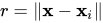
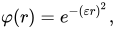
Commonly used types of radial basis functions include (writing ${\textstyle r=\left\|\mathbf {x} -\mathbf {x} _{i}\right\|$ and using ${\textstyle \varepsilon$ to indicate a shape parameter that can be used to scale the input of the radial kernel):

Infinitely Smooth RBFs

These radial basis functions are from $C^{\infty }(\mathbb {R} )$ and are strictly positive-definite functions that require tuning a shape parameter $\varepsilon$
- Gaussian:
  $\varphi (r)=e^{-(\varepsilon r)^{2}},$ 2
- Inverse quadratic:
  $\varphi (r)={\dfrac {1}{1+(\varepsilon r)^{2}}},$ 3
- Inverse multiquadric:
  $\varphi (r)={\dfrac {1}{\sqrt {1+(\varepsilon r)^{2}}}},$ 4
Other Infinitely Smooth RBFs

These radial basis functions are also from $C^{\infty }(\mathbb {R} )$ and require tuning a shape parameter $\varepsilon$ , but they are not strictly positive definite.
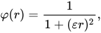
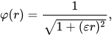
- Multiquadric:
  $\varphi (r)={\sqrt {1+(\varepsilon r)^{2}}},$ 5
- RTH:
  $\varphi (r)=r\tanh(\varepsilon r),$ 6
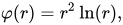
Polyharmonic spline:
${\begin{aligned}\varphi (r)&=r^{k},&k&=1,3,5,\dotsc \\\varphi (r)&=r^{k}\ln(r),&k&=2,4,6,\dotsc \end{aligned}}$ 7
*For even-degree polyharmonic splines $(k=2,4,6,\dotsc )$ , to avoid numerical problems at $r=0$ where $\ln(0)=-\infty$ , the computational implementation is often written as $\varphi (r)=r^{k-1}\ln(r^{r})$ .
Thin plate spline (a special polyharmonic spline):
$\varphi (r)=r^{2}\ln(r),$ 8
Compactly Supported RBFs

These RBFs are compactly supported and thus are non-zero only within a radius of $1/\varepsilon$ , and thus have sparse differentiation matrices
- Bump function:
  $\varphi (r)={\begin{cases}\exp \left(-{\frac {1}{1-(\varepsilon r)^{2}}}\right)&{\text{ for }}r<{\frac {1}{\varepsilon }}\\0&{\text{ otherwise}}\end{cases}},$ 9

02Approximation

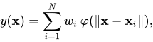
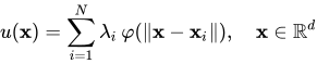
Radial basis functions are typically used to build up function approximations of the form

y(\mathbf {x} )=\sum _{i=1}^{N}w_{i}\,\varphi (\left\|\mathbf {x} -\mathbf {x} _{i}\right\|),

where the approximating function ${\textstyle y(\mathbf {x} )$ is represented as a sum of $N$ radial basis functions, each associated with a different center ${\textstyle \mathbf {x} _{i}$ , and weighted by an appropriate coefficient ${\textstyle w_{i}.$ The weights ${\textstyle w_{i}$ can be estimated using the matrix methods of linear least squares, because the approximating function is linear in the weights ${\textstyle w_{i}$ .

Approximation schemes of this kind have been particularly used in time series prediction and control of nonlinear systems exhibiting sufficiently simple chaotic behaviour and 3D reconstruction in computer graphics (for example, hierarchical RBF and Pose Space Deformation).

Comparison of RTH, Multiquadric (ε = 2), and Linear RBFs

03RBF Network

The sum

y(\mathbf {x} )=\sum _{i=1}^{N}w_{i}\,\varphi (\left\|\mathbf {x} -\mathbf {x} _{i}\right\|),

can also be interpreted as a rather simple single-layer type of artificial neural network called a radial basis function network, with the radial basis functions taking on the role of the activation functions of the network. It can be shown that any continuous function on a compact interval can in principle be interpolated with arbitrary accuracy by a sum of this form, if a sufficiently large number ${\textstyle N$ of radial basis functions is used.

The approximant ${\textstyle y(\mathbf {x} )$ is differentiable with respect to the weights ${\textstyle w_{i}$ . The weights could thus be learned using any of the standard iterative methods for neural networks.

Using radial basis functions in this manner yields a reasonable interpolation approach provided that the fitting set has been chosen such that it covers the entire range systematically (equidistant data points are ideal). However, without a polynomial term that is orthogonal to the radial basis functions, estimates outside the fitting set tend to perform poorly.

04RBFs for PDEs

Radial basis functions are used to approximate functions and so can be used to discretize and numerically solve Partial Differential Equations (PDEs). This was first done in 1990 by E. J. Kansa who developed the first RBF based numerical method. It is called the Kansa method and was used to solve the elliptic Poisson equation and the linear advection-diffusion equation. The function values at points $\mathbf {x}$ in the domain are approximated by the linear combination of RBFs:

u(\mathbf {x} )=\sum _{i=1}^{N}\lambda _{i}\,\varphi (\left\|\mathbf {x} -\mathbf {x} _{i}\right\|),\quad \mathbf {x} \in \mathbb {R} ^{d}

The derivatives are approximated as such:

{\frac {\partial ^{n}u({\textbf {x}})}{\partial x^{n}}}=\sum _{i=1}^{N}\lambda _{i}\,{\frac {\partial ^{n}}{\partial x^{n}}}\varphi (\left\|\mathbf {x} -\mathbf {x} _{i}\right\|),\quad \mathbf {x} \in \mathbb {R} ^{d}

where $N$ are the number of points in the discretized domain, $d$ the dimension of the domain and $\lambda$ the scalar coefficients that are unchanged by the differential operator.

Different numerical methods based on Radial Basis Functions were developed thereafter. Some methods are the RBF-FD method, the RBF-QR method and the RBF-PUM method.

Watch videos about Radial basis functionExplainers and documentaries on YouTube (opens in a new tab)

Sources and credits

This article is adapted from the Wikipedia article “Radial basis function”, written by its contributors and licensed under CC BY-SA 4.0. Fathomly has changed the layout, removed citation markers, navigation and maintenance notices, and adjusted punctuation. This adapted version is shared under the same license. For references, see the original article.

Images, from Wikimedia Commons:

Gaussian function shape parameter.png by Shawsa7, CC BY-SA 4.0
WiKipic1new.svg by MHeidari3, CC BY-SA 4.0
Bump function shape.png by Shawsa7, CC BY-SA 4.0
Unnormalized radial basis functions.svg by Pac72, Public domain

Fathomly is not affiliated with or endorsed by the Wikimedia Foundation. Spotted a problem? Tell us.

Radial basis function

01Definition

Examples

02Approximation

03RBF Network

04RBFs for PDEs

Sources and credits

Related topics

Matérn covariance function

Radial basis function interpolation

Kansa method