Reference articles on history, science, culture and more
Encyclopedia

Weighted least squares

Method for model fitting in statistics

Weighted least squares (WLS), also known as weighted linear regression, is a generalization of ordinary least squares and linear regression in which knowledge of the unequal variance of observations (heteroscedasticity) is incorporated into the regression. WLS is also a specialization of generalized least squares, when all the off-diagonal entries of the covariance matrix of the errors are null.

01Formulation

The fit of a model to a data point is measured by its residual, r_{i}, defined as the difference between a measured value of the dependent variable, y_{i} and the value predicted by the model, f(x_{i},{\boldsymbol {\beta }}): r_{i}({\boldsymbol {\beta }})=y_{i}-f(x_{i},{\boldsymbol {\beta }}).

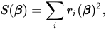
If the errors are uncorrelated and have equal variance, then the function S({\boldsymbol {\beta }})=\sum _{i}r_{i}({\boldsymbol {\beta }})^{2}, is minimized at {\boldsymbol {\hat {\beta }}}, such that {\frac {\partial S}{\partial \beta _{j}}}({\hat {\boldsymbol {\beta }}})=0.
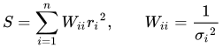
The Gauss-Markov theorem shows that, when this is so, {\hat {\boldsymbol {\beta }}} is a best linear unbiased estimator (BLUE). If, however, the measurements are uncorrelated but have different uncertainties, a modified approach might be adopted. Aitken showed that when a weighted sum of squared residuals is minimized, {\hat {\boldsymbol {\beta }}} is the BLUE if each weight is equal to the reciprocal of the variance of the measurement {\begin{aligned}S&=\sum _{i=1}^{n}W_{ii}{r_{i}}^{2},&W_{ii}&={\frac {1}{{\sigma _{i}}^{2}}}\end{aligned}}

The gradient equations for this sum of squares are -2\sum _{i}W_{ii}{\frac {\partial f(x_{i},{\boldsymbol {\beta }})}{\partial \beta _{j}}}r_{i}=0,\quad j=1,\ldots ,m

which, in a linear least squares system give the modified normal equations, \sum _{i=1}^{n}\sum _{k=1}^{m}X_{ij}W_{ii}X_{ik}{\hat {\beta }}_{k}=\sum _{i=1}^{n}X_{ij}W_{ii}y_{i},\quad j=1,\ldots ,m\,. The matrix X above is as defined in the corresponding discussion of linear least squares.

When the observational errors are uncorrelated and the weight matrix, W=Ω−1, is diagonal, these may be written as \mathbf {\left(X^{\textsf {T}}WX\right){\hat {\boldsymbol {\beta }}}=X^{\textsf {T}}Wy} .

If the errors are correlated, the resulting estimator is the BLUE if the weight matrix is equal to the inverse of the variance-covariance matrix of the observations.

When the errors are uncorrelated, it is convenient to simplify the calculations to factor the weight matrix as w_{ii}={\sqrt {W_{ii}}}. The normal equations can then be written in the same form as ordinary least squares: \mathbf {\left(X'^{\textsf {T}}X'\right){\hat {\boldsymbol {\beta }}}=X'^{\textsf {T}}y'} \,

where we define the following scaled matrix and vector: {\begin{aligned}\mathbf {X'} &=\operatorname {diag} \left(\mathbf {w} \right)\mathbf {X} ,\\\mathbf {y'} &=\operatorname {diag} \left(\mathbf {w} \right)\mathbf {y} =\mathbf {y} \oslash \mathbf {\sigma } .\end{aligned}}
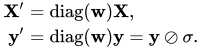
This is a type of whitening transformation; the last expression involves an entrywise division.

For non-linear least squares systems a similar argument shows that the normal equations should be modified as follows. \mathbf {\left(J^{\textsf {T}}WJ\right)\,{\boldsymbol {\Delta }}\beta =J^{\textsf {T}}W\,{\boldsymbol {\Delta }}y} .\,

Note that for empirical tests, the appropriate W is not known for sure and must be estimated. For this feasible generalized least squares (FGLS) techniques may be used; in this case it is specialized for a diagonal covariance matrix, thus yielding a feasible weighted least squares solution.

If the uncertainty of the observations is not known from external sources, then the weights could be estimated from the given observations. This can be useful, for example, to identify outliers. After the outliers have been removed from the data set, the weights should be reset to one.

02Motivation

In some cases the observations may be weighted, for example, they may not be equally reliable. In this case, one can minimize the weighted sum of squares: {\underset {\boldsymbol {\beta }}{\operatorname {arg\ min} }}\,\sum _{i=1}^{n}w_{i}\left|y_{i}-\sum _{j=1}^{m}X_{ij}\beta _{j}\right|^{2}={\underset {\boldsymbol {\beta }}{\operatorname {arg\ min} }}\,\left\|W^{\frac {1}{2}}\left(\mathbf {y} -X{\boldsymbol {\beta }}\right)\right\|^{2}. where wi > 0 is the weight of the ith observation, and W is the diagonal matrix of such weights.

The weights should, ideally, be equal to the reciprocal of the variance of the measurement. (This implies that the observations are uncorrelated. If the observations are correlated, the expression {\textstyle S=\sum _{k}\sum _{j}r_{k}W_{kj}r_{j}\, applies. In this case the weight matrix should ideally be equal to the inverse of the variance-covariance matrix of the observations). The normal equations are then: \left(X^{\textsf {T}}WX\right){\hat {\boldsymbol {\beta }}}=X^{\textsf {T}}W\mathbf {y} .

This method is used in iteratively reweighted least squares.

03Solution

Parameter errors and correlation

The estimated parameter values are linear combinations of the observed values {\hat {\boldsymbol {\beta }}}=(X^{\textsf {T}}WX)^{-1}X^{\textsf {T}}W\mathbf {y} .

Therefore, an expression for the estimated variance-covariance matrix of the parameter estimates can be obtained by error propagation from the errors in the observations. Let the variance-covariance matrix for the observations be denoted by M and that of the estimated parameters by Mβ. Then M^{\beta }=\left(X^{\textsf {T}}WX\right)^{-1}X^{\textsf {T}}WMW^{\textsf {T}}X\left(X^{\textsf {T}}W^{\textsf {T}}X\right)^{-1}.

When W = M−1, this simplifies to M^{\beta }=\left(X^{\textsf {T}}WX\right)^{-1}.

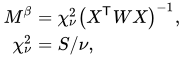
When unit weights are used (W = I, the identity matrix), it is implied that the experimental errors are uncorrelated and all equal: M = σ2I, where σ2 is the a priori variance of an observation. In any case, σ2 is approximated by the reduced chi-squared \chi _{\nu }^{2}: {\begin{aligned}M^{\beta }&=\chi _{\nu }^{2}\left(X^{\textsf {T}}WX\right)^{-1},\\\chi _{\nu }^{2}&=S/\nu ,\end{aligned}}

where S is the minimum value of the weighted objective function: S=r^{\textsf {T}}Wr=\left\|W^{\frac {1}{2}}\left(\mathbf {y} -X{\hat {\boldsymbol {\beta }}}\right)\right\|^{2}.

The denominator, \nu =n-m, is the number of degrees of freedom; see effective degrees of freedom for generalizations for the case of correlated observations.

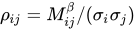
In all cases, the variance of the parameter estimate {\hat {\beta }}_{i} is given by M_{ii}^{\beta } and the covariance between the parameter estimates {\hat {\beta }}_{i} and {\hat {\beta }}_{j} is given by M_{ij}^{\beta }. The standard deviation is the square root of variance, \sigma _{i}={\sqrt {M_{ii}^{\beta }}}, and the correlation coefficient is given by \rho _{ij}=M_{ij}^{\beta }/(\sigma _{i}\sigma _{j}). These error estimates reflect only random errors in the measurements. The true uncertainty in the parameters is larger due to the presence of systematic errors, which, by definition, cannot be quantified. Note that even though the observations may be uncorrelated, the parameters are typically correlated.

Parameter confidence limits

It is often assumed, for want of any concrete evidence but often appealing to the central limit theorem, see Normal distribution#Occurrence and applications, that the error on each observation belongs to a normal distribution with a mean of zero and standard deviation \sigma. Under that assumption the following probabilities can be derived for a single scalar parameter estimate in terms of its estimated standard error se_{\beta } (given here):

  • 68% that the interval {\hat {\beta }}\pm se_{\beta } encompasses the true coefficient value
  • 95% that the interval {\hat {\beta }}\pm 2se_{\beta } encompasses the true coefficient value
  • 99% that the interval {\hat {\beta }}\pm 2.5se_{\beta } encompasses the true coefficient value

The assumption is not unreasonable when n >> m. If the experimental errors are normally distributed the parameters will belong to a Student's t-distribution with n  m degrees of freedom. When n  m Student's t-distribution approximates a normal distribution. Note, however, that these confidence limits cannot take systematic error into account. Also, parameter errors should be quoted to one significant figure only, as they are subject to sampling error.

When the number of observations is relatively small, Chebychev's inequality can be used for an upper bound on probabilities, regardless of any assumptions about the distribution of experimental errors: the maximum probabilities that a parameter will be more than 1, 2, or 3 standard deviations away from its expectation value are 100%, 25% and 11% respectively.

Residual values and correlation

The residuals are related to the observations by \mathbf {\hat {r}} =\mathbf {y} -X{\hat {\boldsymbol {\beta }}}=\mathbf {y} -H\mathbf {y} =(I-H)\mathbf {y} ,

where H is the idempotent matrix known as the hat matrix: H=X\left(X^{\textsf {T}}WX\right)^{-1}X^{\textsf {T}}W,

and I is the identity matrix. The variance-covariance matrix of the residuals, M r is given by M^{\mathbf {r} }=(I-H)M(I-H)^{\textsf {T}}.

Thus the residuals are correlated, even if the observations are not.

When W=M^{-1}, M^{\mathbf {r} }=(I-H)M.

The sum of weighted residual values is equal to zero whenever the model function contains a constant term. Left-multiply the expression for the residuals by XT WT: X^{\textsf {T}}W{\hat {\mathbf {r} }}=X^{\textsf {T}}W\mathbf {y} -X^{\textsf {T}}WX{\hat {\boldsymbol {\beta }}}=X^{\textsf {T}}W\mathbf {y} -\left(X^{\rm {T}}WX\right)\left(X^{\textsf {T}}WX\right)^{-1}X^{\textsf {T}}W\mathbf {y} =\mathbf {0} .

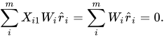
Say, for example, that the first term of the model is a constant, so that X_{i1}=1 for all i. In that case it follows that \sum _{i}^{m}X_{i1}W_{i}{\hat {r}}_{i}=\sum _{i}^{m}W_{i}{\hat {r}}_{i}=0.

Thus, in the motivational example, above, the fact that the sum of residual values is equal to zero is not accidental, but is a consequence of the presence of the constant term, α, in the model.

If experimental error follows a normal distribution, then, because of the linear relationship between residuals and observations, so should residuals, but since the observations are only a sample of the population of all possible observations, the residuals should belong to a Student's t-distribution. Studentized residuals are useful in making a statistical test for an outlier when a particular residual appears to be excessively large.

Watch videos about Weighted least squaresExplainers and documentaries on YouTube (opens in a new tab)

Sources and credits

This article is adapted from the Wikipedia article Weighted least squares, written by its contributors and licensed under CC BY-SA 4.0. Fathomly has changed the layout, removed citation markers, navigation and maintenance notices, and adjusted punctuation. This adapted version is shared under the same license. For references, see the original article.

Fathomly is not affiliated with or endorsed by the Wikimedia Foundation. Spotted a problem? Tell us.

Continue exploring

Related topics

Iteratively reweighted least squares

The method of iteratively reweighted least squares is used to solve certain optimization problems with objective functions of the form of a p-norm, a r g m i n β ⁡ ∑ i = 1 n | y i − f i ( β ) | p , {\displaystyle \operatorname {arg\,min} _{\boldsymbol {\beta }}\sum _{i=1}^{n}{\big |}y_{i}-f_{i}({\boldsymbol {\beta }}){\big |}^{p},} by an iterative method in which each step involves solving a weighted least squares problem of the form β ( t + 1 ) = a r g m i n β ⁡ ∑ i = 1 n w i ( β ( t ) ) | y i − f i ( β ) | 2 . {\displaystyle {\boldsymbol {\beta }}^{(t+1)}=\operatorname {arg\,min} _{\boldsymbol {\beta }}\sum _{i=1}^{n}w_{i}({\boldsymbol {\beta }}^{(t)}){\big |}y_{i}-f_{i}({\boldsymbol {\beta }}){\big |}^{2}.} IRLS is used to find the maximum likelihood estimates of a generalized linear model, and in robust regression to find an M-estimator, as a way of mitigating the influence of outliers in an otherwise normally distributed data set, for example, by minimizing the least absolute errors rather than the least square errors.

Heteroskedasticity-consistent standard errors

The topic of heteroskedasticity-consistent standard errors arises in statistics and econometrics in the context of linear regression and time series analysis. These are also known as heteroskedasticity-robust standard errors (or simply robust standard errors), Eicker-Huber-White standard errors (also Huber-White standard errors or White standard errors), to recognize the contributions of Friedhelm Eicker, Peter J. Huber, and Halbert White.

Weighted arithmetic mean

The weighted arithmetic mean is similar to an ordinary arithmetic mean, except that instead of each of the data points contributing equally to the final average, some data points contribute more than others. The notion of weighted mean plays a role in descriptive statistics and also occurs in a more general form in several other areas of mathematics.