Encyclopedia

Propagation of uncertainty

Effect of variables' uncertainties on the uncertainty of a function based on them

Wikipedia contributorsAdapted for Fathomly · View authors

7 min read
Source updated January 10, 2026

In statistics, propagation of uncertainty is the effect of variables' uncertainties on the uncertainty of a function based on them. When the variables are the values of experimental measurements they have uncertainties due to measurement limitations (e.g., instrument precision) which propagate due to the combination of variables in the function.

The uncertainty u can be expressed in a number of ways. It may be defined by the absolute error Δx. Uncertainties can also be defined by the relative error (Δx)/x, which is usually written as a percentage. Most commonly, the uncertainty on a quantity is quantified in terms of the standard deviation, σ, which is the positive square root of the variance. The value of a quantity and its error are then expressed as an interval x ± u. However, the most general way of characterizing uncertainty is by specifying its probability distribution. If the probability distribution of the variable is known or can be assumed, in theory it is possible to get any of its statistics. In particular, it is possible to derive confidence limits to describe the region within which the true value of the variable may be found. For example, the 68% confidence limits for a one-dimensional variable belonging to a normal distribution are approximately ± one standard deviation σ from the central value x, which means that the region x ± σ will cover the true value in roughly 68% of cases.

If the uncertainties are correlated then covariance must be taken into account. Correlation can arise from two different sources. First, the measurement errors may be correlated. Second, when the underlying values are correlated across a population, the uncertainties in the group averages will be correlated.

In a general context where a nonlinear function modifies the uncertain parameters (correlated or not), the standard tools to propagate uncertainty, and infer resulting quantity probability distribution/statistics, are sampling techniques from the Monte Carlo method family. For very large datasets or complex functions, the calculation of the error propagation may be very expensive so that a surrogate model or a parallel computing strategy may be necessary.

In some particular cases, the uncertainty propagation calculation can be done through simplistic algebraic procedures. Some of these scenarios are described below.

01Linear combinations

Let $\{f_{k}(x_{1},x_{2},\dots ,x_{n})\}$ be a set of m functions, which are linear combinations of $n$ variables $x_{1},x_{2},\dots ,x_{n}$ with combination coefficients $A_{k1},A_{k2},\dots ,A_{kn},(k=1,\dots ,m)$ : $f_{k}=\sum _{i=1}^{n}A_{ki}x_{i},$ or in matrix notation, $\mathbf {f} =\mathbf {A} \mathbf {x} .$

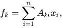
Also let the variance-covariance matrix of x = (x₁, ..., x_n) be denoted by ${\boldsymbol {\Sigma }}^{x}$ and let the mean value be denoted by ${\boldsymbol {\mu }}$ : ${\begin{aligned}{\boldsymbol {\Sigma }}^{x}=\operatorname {E} [(\mathbf {x} -{\boldsymbol {\mu }})\otimes (\mathbf {x} -{\boldsymbol {\mu }})]&={\begin{pmatrix}\sigma _{1}^{2}&\sigma _{12}&\sigma _{13}&\cdots \\\sigma _{21}&\sigma _{2}^{2}&\sigma _{23}&\cdots \\\sigma _{31}&\sigma _{32}&\sigma _{3}^{2}&\cdots \\\vdots &\vdots &\vdots &\ddots \end{pmatrix}}\\[1ex]&={\begin{pmatrix}{\Sigma }_{11}^{x}&{\Sigma }_{12}^{x}&{\Sigma }_{13}^{x}&\cdots \\{\Sigma }_{21}^{x}&{\Sigma }_{22}^{x}&{\Sigma }_{23}^{x}&\cdots \\{\Sigma }_{31}^{x}&{\Sigma }_{32}^{x}&{\Sigma }_{33}^{x}&\cdots \\\vdots &\vdots &\vdots &\ddots \end{pmatrix}}.\end{aligned}}$ $\otimes$ is the outer product.

Then, the variance-covariance matrix ${\boldsymbol {\Sigma }}^{f}$ of f is given by ${\begin{aligned}{\boldsymbol {\Sigma }}^{f}&=\operatorname {E} \left[(\mathbf {f} -\operatorname {E} [\mathbf {f} ])\otimes (\mathbf {f} -\operatorname {E} [\mathbf {f} ])\right]=\operatorname {E} \left[\mathbf {A} (\mathbf {x} -{\boldsymbol {\mu }})\otimes \mathbf {A} (\mathbf {x} -{\boldsymbol {\mu }})\right]\\[1ex]&=\mathbf {A} \operatorname {E} \left[(\mathbf {x} -{\boldsymbol {\mu }})\otimes (\mathbf {x} -{\boldsymbol {\mu }})\right]\mathbf {A} ^{\mathrm {T} }=\mathbf {A} {\boldsymbol {\Sigma }}^{x}\mathbf {A} ^{\mathrm {T} }.\end{aligned}}$

In component notation, the equation ${\boldsymbol {\Sigma }}^{f}=\mathbf {A} {\boldsymbol {\Sigma }}^{x}\mathbf {A} ^{\mathrm {T} }$ reads $\Sigma _{ij}^{f}=\sum _{k}^{n}\sum _{l}^{n}A_{ik}{\Sigma }_{kl}^{x}A_{jl}.$

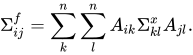
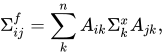
This is the most general expression for the propagation of error from one set of variables onto another. When the errors on x are uncorrelated, the general expression simplifies to $\Sigma _{ij}^{f}=\sum _{k}^{n}A_{ik}\Sigma _{k}^{x}A_{jk},$ where $\Sigma _{k}^{x}=\sigma _{x_{k}}^{2}$ is the variance of k-th element of the x vector. Note that even though the errors on x may be uncorrelated, the errors on f are in general correlated; in other words, even if ${\boldsymbol {\Sigma }}^{x}$ is a diagonal matrix, ${\boldsymbol {\Sigma }}^{f}$ is in general a full matrix.

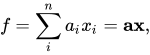
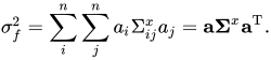
The general expressions for a scalar-valued function f are a little simpler (here a is a row vector): $f=\sum _{i}^{n}a_{i}x_{i}=\mathbf {ax} ,$ $\sigma _{f}^{2}=\sum _{i}^{n}\sum _{j}^{n}a_{i}\Sigma _{ij}^{x}a_{j}=\mathbf {a} {\boldsymbol {\Sigma }}^{x}\mathbf {a} ^{\mathrm {T} }.$

Each covariance term $\sigma _{ij}$ can be expressed in terms of the correlation coefficient $\rho _{ij}$ by $\sigma _{ij}=\rho _{ij}\sigma _{i}\sigma _{j}$ , so that an alternative expression for the variance of f is $\sigma _{f}^{2}=\sum _{i}^{n}a_{i}^{2}\sigma _{i}^{2}+\sum _{i}^{n}\sum _{j(j\neq i)}^{n}a_{i}a_{j}\rho _{ij}\sigma _{i}\sigma _{j}.$

In the case that the variables in x are uncorrelated, this simplifies further to $\sigma _{f}^{2}=\sum _{i}^{n}a_{i}^{2}\sigma _{i}^{2}.$

In the simple case of identical coefficients and variances, we find $\sigma _{f}={\sqrt {n}}\,|a|\sigma .$

For the arithmetic mean, $a=1/n$ , the result is the standard error of the mean: $\sigma _{f}={\frac {\sigma }{\sqrt {n}}}.$

02Non-linear combinations

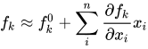
When f is a set of non-linear combination of the variables x, an interval propagation could be performed in order to compute intervals which contain all consistent values for the variables. In a probabilistic approach, the function f must usually be linearised by approximation to a first-order Taylor series expansion, though in some cases, exact formulae can be derived that do not depend on the expansion as is the case for the exact variance of products. The Taylor expansion would be: $f_{k}\approx f_{k}^{0}+\sum _{i}^{n}{\frac {\partial f_{k}}{\partial {x_{i}}}}x_{i}$ where $\partial f_{k}/\partial x_{i}$ denotes the partial derivative of f_k with respect to the i-th variable, evaluated at the mean value of all components of vector x. Or in matrix notation, $\mathrm {f} \approx \mathrm {f} ^{0}+\mathrm {J} \mathrm {x} \,$ where J is the Jacobian matrix. Since f⁰ is a constant it does not contribute to the error on f. Therefore, the propagation of error follows the linear case, above, but replacing the linear coefficients, A_ki and A_kj by the partial derivatives, ${\frac {\partial f_{k}}{\partial x_{i}}}$ and ${\frac {\partial f_{k}}{\partial x_{j}}}$ . In matrix notation, $\mathrm {\Sigma } ^{\mathrm {f} }=\mathrm {J} \mathrm {\Sigma } ^{\mathrm {x} }\mathrm {J} ^{\top }.$

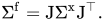
That is, the Jacobian of the function is used to transform the rows and columns of the variance-covariance matrix of the argument. Note this is equivalent to the matrix expression for the linear case with $\mathrm {J=A}$ .

Simplification

Neglecting correlations or assuming independent variables yields a common formula among engineers and experimental scientists to calculate error propagation, the variance formula: $s_{f}={\sqrt {\left({\frac {\partial f}{\partial x}}\right)^{2}s_{x}^{2}+\left({\frac {\partial f}{\partial y}}\right)^{2}s_{y}^{2}+\left({\frac {\partial f}{\partial z}}\right)^{2}s_{z}^{2}+\cdots }}$ where $s_{f}$ represents the standard deviation of the function $f$ , $s_{x}$ represents the standard deviation of $x$ , $s_{y}$ represents the standard deviation of $y$ , and so forth.

This formula is based on the linear characteristics of the gradient of $f$ and therefore it is a good estimation for the standard deviation of $f$ as long as $s_{x},s_{y},s_{z},\ldots$ are small enough. Specifically, the linear approximation of $f$ has to be close to $f$ inside a neighbourhood of radius $s_{x},s_{y},s_{z},\ldots$ .

Example

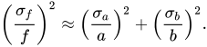
Any non-linear differentiable function, $f(a,b)$ , of two variables, $a$ and $b$ , can be expanded as $f\approx f^{0}+{\frac {\partial f}{\partial a}}a+{\frac {\partial f}{\partial b}}b.$ If we take the variance on both sides and use the formula for the variance of a linear combination of variables $\operatorname {Var} (aX+bY)=a^{2}\operatorname {Var} (X)+b^{2}\operatorname {Var} (Y)+2ab\operatorname {Cov} (X,Y),$ then we obtain $\sigma _{f}^{2}\approx \left|{\frac {\partial f}{\partial a}}\right|^{2}\sigma _{a}^{2}+\left|{\frac {\partial f}{\partial b}}\right|^{2}\sigma _{b}^{2}+2{\frac {\partial f}{\partial a}}{\frac {\partial f}{\partial b}}\sigma _{ab},$ where $\sigma _{f}$ is the standard deviation of the function $f$ , $\sigma _{a}$ is the standard deviation of $a$ , $\sigma _{b}$ is the standard deviation of $b$ and $\sigma _{ab}=\sigma _{a}\sigma _{b}\rho _{ab}$ is the covariance between $a$ and $b$ .

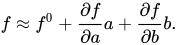
In the particular case that $f=ab$ , ${\frac {\partial f}{\partial a}}=b$ , ${\frac {\partial f}{\partial b}}=a$ . Then $\sigma _{f}^{2}\approx b^{2}\sigma _{a}^{2}+a^{2}\sigma _{b}^{2}+2ab\,\sigma _{ab}$ or $\left({\frac {\sigma _{f}}{f}}\right)^{2}\approx \left({\frac {\sigma _{a}}{a}}\right)^{2}+\left({\frac {\sigma _{b}}{b}}\right)^{2}+2\left({\frac {\sigma _{a}}{a}}\right)\left({\frac {\sigma _{b}}{b}}\right)\rho _{ab}$ where $\rho _{ab}$ is the correlation between $a$ and $b$ .

When the variables $a$ and $b$ are uncorrelated, $\rho _{ab}=0$ . Then $\left({\frac {\sigma _{f}}{f}}\right)^{2}\approx \left({\frac {\sigma _{a}}{a}}\right)^{2}+\left({\frac {\sigma _{b}}{b}}\right)^{2}.$

Caveats and warnings

Error estimates for non-linear functions are biased on account of using a truncated series expansion. The extent of this bias depends on the nature of the function. For example, the bias on the error calculated for log(1+x) increases as x increases, since the expansion to x is a good approximation only when x is near zero.

For highly non-linear functions, there exist five categories of probabilistic approaches for uncertainty propagation; see Uncertainty quantification for details.

Reciprocal and shifted reciprocal

In the special case of the inverse or reciprocal $1/B$ , where $B=N(0,1)$ follows a standard normal distribution, the resulting distribution is a reciprocal standard normal distribution, and there is no definable variance.

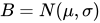
However, in the slightly more general case of a shifted reciprocal function $1/(p-B)$ for $B=N(\mu ,\sigma )$ following a general normal distribution, then mean and variance statistics do exist in a principal value sense, if the difference between the pole $p$ and the mean $\mu$ is real-valued.

Ratios

Ratios are also problematic; normal approximations exist under certain conditions.

03Example formulae

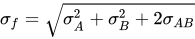
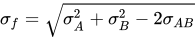
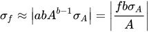
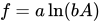
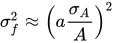
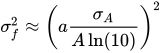
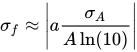
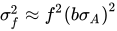
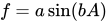
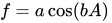
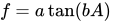
This table shows the variances and standard deviations of simple functions of the real variables $A,B$ with standard deviations $\sigma _{A},\sigma _{B},$ covariance $\sigma _{AB}=\rho _{AB}\sigma _{A}\sigma _{B},$ and correlation $\rho _{AB}.$ The real-valued coefficients $a$ and $b$ are assumed exactly known (deterministic), i.e., $\sigma _{a}=\sigma _{b}=0.$

In the right-hand columns of the table, $A$ and $B$ are expectation values, and $f$ is the value of the function calculated at those values.

Function	Variance	Standard deviation
$f=aA\,$	$\sigma _{f}^{2}=a^{2}\sigma _{A}^{2}$	$\sigma _{f}=\|a\|\sigma _{A}$
$f=A+B$	$\sigma _{f}^{2}=\sigma _{A}^{2}+\sigma _{B}^{2}+2\sigma _{AB}$	$\sigma _{f}={\sqrt {\sigma _{A}^{2}+\sigma _{B}^{2}+2\sigma _{AB}}}$
$f=A-B$	$\sigma _{f}^{2}=\sigma _{A}^{2}+\sigma _{B}^{2}-2\sigma _{AB}$	$\sigma _{f}={\sqrt {\sigma _{A}^{2}+\sigma _{B}^{2}-2\sigma _{AB}}}$
$f=aA+bB$	$\sigma _{f}^{2}=a^{2}\sigma _{A}^{2}+b^{2}\sigma _{B}^{2}+2ab\,\sigma _{AB}$	$\sigma _{f}={\sqrt {a^{2}\sigma _{A}^{2}+b^{2}\sigma _{B}^{2}+2ab\,\sigma _{AB}}}$
$f=aA-bB$	$\sigma _{f}^{2}=a^{2}\sigma _{A}^{2}+b^{2}\sigma _{B}^{2}-2ab\,\sigma _{AB}$	$\sigma _{f}={\sqrt {a^{2}\sigma _{A}^{2}+b^{2}\sigma _{B}^{2}-2ab\,\sigma _{AB}}}$
$f=AB$	$\sigma _{f}^{2}\approx f^{2}\left[\left({\frac {\sigma _{A}}{A}}\right)^{2}+\left({\frac {\sigma _{B}}{B}}\right)^{2}+2{\frac {\sigma _{AB}}{AB}}\right]$	$\sigma _{f}\approx \left\|f\right\|{\sqrt {\left({\frac {\sigma _{A}}{A}}\right)^{2}+\left({\frac {\sigma _{B}}{B}}\right)^{2}+2{\frac {\sigma _{AB}}{AB}}}}$
$f={\frac {A}{B}}$	$\sigma _{f}^{2}\approx f^{2}\left[\left({\frac {\sigma _{A}}{A}}\right)^{2}+\left({\frac {\sigma _{B}}{B}}\right)^{2}-2{\frac {\sigma _{AB}}{AB}}\right]$	$\sigma _{f}\approx \left\|f\right\|{\sqrt {\left({\frac {\sigma _{A}}{A}}\right)^{2}+\left({\frac {\sigma _{B}}{B}}\right)^{2}-2{\frac {\sigma _{AB}}{AB}}}}$
$f={\frac {A}{A+B}}$	$\sigma _{f}^{2}\approx {\frac {f^{2}}{\left(A+B\right)^{2}}}\left({\frac {B^{2}}{A^{2}}}\sigma _{A}^{2}+\sigma _{B}^{2}-2{\frac {B}{A}}\sigma _{AB}\right)$	$\sigma _{f}\approx \left\|{\frac {f}{A+B}}\right\|{\sqrt {{\frac {B^{2}}{A^{2}}}\sigma _{A}^{2}+\sigma _{B}^{2}-2{\frac {B}{A}}\sigma _{AB}}}$
$f=aA^{b}$	$\sigma _{f}^{2}\approx \left({a}{b}{A}^{b-1}{\sigma _{A}}\right)^{2}=\left({\frac {{f}{b}{\sigma _{A}}}{A}}\right)^{2}$	$\sigma _{f}\approx \left\|{a}{b}{A}^{b-1}{\sigma _{A}}\right\|=\left\|{\frac {{f}{b}{\sigma _{A}}}{A}}\right\|$
$f=a\ln(bA)$	$\sigma _{f}^{2}\approx \left(a{\frac {\sigma _{A}}{A}}\right)^{2}$	$\sigma _{f}\approx \left\|a{\frac {\sigma _{A}}{A}}\right\|$
$f=a\log _{10}(bA)$	$\sigma _{f}^{2}\approx \left(a{\frac {\sigma _{A}}{A\ln(10)}}\right)^{2}$	$\sigma _{f}\approx \left\|a{\frac {\sigma _{A}}{A\ln(10)}}\right\|$
$f=ae^{bA}$	$\sigma _{f}^{2}\approx f^{2}\left(b\sigma _{A}\right)^{2}$	$\sigma _{f}\approx \left\|f\right\|\left\|\left(b\sigma _{A}\right)\right\|$
$f=a^{bA}$	$\sigma _{f}^{2}\approx f^{2}(b\ln(a)\sigma _{A})^{2}$	$\sigma _{f}\approx \left\|f\right\|\left\|b\ln(a)\sigma _{A}\right\|$
$f=a\sin(bA)$	$\sigma _{f}^{2}\approx \left[ab\cos(bA)\sigma _{A}\right]^{2}$	$\sigma _{f}\approx \left\|ab\cos(bA)\sigma _{A}\right\|$
$f=a\cos \left(bA\right)\,$	$\sigma _{f}^{2}\approx \left[ab\sin(bA)\sigma _{A}\right]^{2}$	$\sigma _{f}\approx \left\|ab\sin(bA)\sigma _{A}\right\|$
$f=a\tan \left(bA\right)\,$	$\sigma _{f}^{2}\approx \left[ab\sec ^{2}(bA)\sigma _{A}\right]^{2}$	$\sigma _{f}\approx \left\|ab\sec ^{2}(bA)\sigma _{A}\right\|$
$f=A^{B}$	$\sigma _{f}^{2}\approx f^{2}\left[\left({\frac {B}{A}}\sigma _{A}\right)^{2}+\left(\ln(A)\sigma _{B}\right)^{2}+2{\frac {B\ln(A)}{A}}\sigma _{AB}\right]$	$\sigma _{f}\approx \left\|f\right\|{\sqrt {\left({\frac {B}{A}}\sigma _{A}\right)^{2}+\left(\ln(A)\sigma _{B}\right)^{2}+2{\frac {B\ln(A)}{A}}\sigma _{AB}}}$
$f={\sqrt {aA^{2}\pm bB^{2}}}$	$\sigma _{f}^{2}\approx \left({\frac {A}{f}}\right)^{2}a^{2}\sigma _{A}^{2}+\left({\frac {B}{f}}\right)^{2}b^{2}\sigma _{B}^{2}\pm 2ab{\frac {AB}{f^{2}}}\,\sigma _{AB}$	$\sigma _{f}\approx {\sqrt {\left({\frac {A}{f}}\right)^{2}a^{2}\sigma _{A}^{2}+\left({\frac {B}{f}}\right)^{2}b^{2}\sigma _{B}^{2}\pm 2ab{\frac {AB}{f^{2}}}\,\sigma _{AB}}}$

For uncorrelated variables ( $\rho _{AB}=0$ , $\sigma _{AB}=0$ ) expressions for more complicated functions can be derived by combining simpler functions. For example, repeated multiplication, assuming no correlation, gives $f=ABC;\qquad \left({\frac {\sigma _{f}}{f}}\right)^{2}\approx \left({\frac {\sigma _{A}}{A}}\right)^{2}+\left({\frac {\sigma _{B}}{B}}\right)^{2}+\left({\frac {\sigma _{C}}{C}}\right)^{2}.$

For the case $f=AB$ we also have Goodman's expression for the exact variance: for the uncorrelated case it is $\operatorname {V} [XY]=\operatorname {E} [X]^{2}\operatorname {V} [Y]+\operatorname {E} [Y]^{2}\operatorname {V} [X]+\operatorname {V} [X]\operatorname {V} [Y],$ and therefore we have $\sigma _{f}^{2}=A^{2}\sigma _{B}^{2}+B^{2}\sigma _{A}^{2}+\sigma _{A}^{2}\sigma _{B}^{2}.$ The last term represents a small correction to the usual formula as can be seen by dividing both sides by $f^{2}=A^{2}B^{2}$ . $\left({\frac {\sigma _{f}}{f}}\right)^{2}=\left({\frac {\sigma _{A}}{A}}\right)^{2}+\left({\frac {\sigma _{B}}{B}}\right)^{2}+\left({\frac {\sigma _{A}\sigma _{B}}{AB}}\right)^{2}.$

Effect of correlation on differences

If A and B are uncorrelated, their difference A − B will have more variance than either of them. An increasing positive correlation ( $\rho _{AB}\to 1$ ) will decrease the variance of the difference, converging to zero variance for perfectly correlated variables with the same variance. On the other hand, a negative correlation ( $\rho _{AB}\to -1$ ) will further increase the variance of the difference, compared to the uncorrelated case.

For example, the self-subtraction f = A − A has zero variance $\sigma _{f}^{2}=0$ only if the variate is perfectly autocorrelated ( $\rho _{A}=1$ ). If A is uncorrelated, $\rho _{A}=0,$ then the output variance is twice the input variance, $\sigma _{f}^{2}=2\sigma _{A}^{2}.$ And if A is perfectly anticorrelated, $\rho _{A}=-1,$ then the input variance is quadrupled in the output, $\sigma _{f}^{2}=4\sigma _{A}^{2}$ (notice $1-\rho _{A}=2$ for f = aA − aA in the table above).

04Example calculations

Inverse tangent function

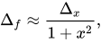
We can calculate the uncertainty propagation for the inverse tangent function as an example of using partial derivatives to propagate error.

Define $f(x)=\arctan(x),$ where $\Delta _{x}$ is the absolute uncertainty on our measurement of x. The derivative of f(x) with respect to x is ${\frac {df}{dx}}={\frac {1}{1+x^{2}}}.$

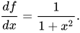
Therefore, our propagated uncertainty is $\Delta _{f}\approx {\frac {\Delta _{x}}{1+x^{2}}},$ where $\Delta _{f}$ is the absolute propagated uncertainty.

Resistance measurement

A practical application is an experiment in which one measures current, I, and voltage, V, on a resistor in order to determine the resistance, R, using Ohm's law, R = V / I.

Given the measured variables with uncertainties, I ± σ_I and V ± σ_V, and neglecting their possible correlation, the uncertainty in the computed quantity, σ_R, is:

$\sigma _{R}\approx {\sqrt {\sigma _{V}^{2}\left({\frac {1}{I}}\right)^{2}+\sigma _{I}^{2}\left({\frac {-V}{I^{2}}}\right)^{2}}}=R{\sqrt {\left({\frac {\sigma _{V}}{V}}\right)^{2}+\left({\frac {\sigma _{I}}{I}}\right)^{2}}}.$

Watch videos about Propagation of uncertaintyExplainers and documentaries on YouTube (opens in a new tab)

Sources and credits

This article is adapted from the Wikipedia article “Propagation of uncertainty”, written by its contributors and licensed under CC BY-SA 4.0. Fathomly has changed the layout, removed citation markers, navigation and maintenance notices, and adjusted punctuation. This adapted version is shared under the same license. For references, see the original article.

Fathomly is not affiliated with or endorsed by the Wikimedia Foundation. Spotted a problem? Tell us.