Uncertainty quantification

There are two major types of problems in uncertainty quantification: one is the forward propagation of uncertainty (where the various sources of uncertainty are propagated through the model to predict the overall uncertainty in the system response) and the other is the inverse assessment of model uncertainty and parameter uncertainty (where the model parameters are calibrated simultaneously using test data). There has been a proliferation of research on the former problem and a majority of uncertainty analysis techniques were developed for it. On the other hand, the latter problem is drawing increasing attention in the engineering design community, since uncertainty quantification of a model and the subsequent predictions of the true system response(s) are of great interest in designing robust systems.

Forward

Uncertainty propagation is the quantification of uncertainties in system output(s) propagated from uncertain inputs. It focuses on the influence on the outputs from the parametric variability listed in the sources of uncertainty. The targets of uncertainty propagation analysis can be:

• To evaluate low-order moments of the outputs, i.e. mean and variance.
• To evaluate the reliability of the outputs. This is especially useful in reliability engineering where outputs of a system are usually closely related to the performance of the system.
• To assess the complete probability distribution of the outputs. This is useful in the scenario of utility optimization where the complete distribution is used to calculate the utility.
• To estimate uncertainty in values, that cannot be directly measured, when calculated with experimentally measurable values. This is especially useful in experimental physics and chemistry contexts.

Inverse

Given some experimental measurements of a system and some computer simulation results from its mathematical model, inverse uncertainty quantification estimates the discrepancy between the experiment and the mathematical model (which is called bias correction), and estimates the values of unknown parameters in the model if there are any (which is called parameter calibration or simply calibration). Generally this is a much more difficult problem than forward uncertainty propagation; however it is of great importance since it is typically implemented in a model updating process. There are several scenarios in inverse uncertainty quantification:

Bias correction only

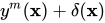
Bias correction quantifies the model inadequacy, i.e. the discrepancy between the experiment and the mathematical model. The general model updating formula for bias correction is:

where denotes the experimental measurements as a function of several input variables , denotes the computer model (mathematical model) response, denotes the additive discrepancy function (aka bias function), and denotes the experimental uncertainty. The objective is to estimate the discrepancy function , and as a by-product, the resulting updated model is . A prediction confidence interval is provided with the updated model as the quantification of the uncertainty.

Parameter calibration only

Parameter calibration estimates the values of one or more unknown parameters in a mathematical model. The general model updating formulation for calibration is:

where denotes the computer model response that depends on several unknown model parameters , and denotes the true values of the unknown parameters in the course of experiments. The objective is to either estimate , or to come up with a probability distribution of that encompasses the best knowledge of the true parameter values.

Bias correction and parameter calibration

It considers an inaccurate model with one or more unknown parameters, and its model updating formulation combines the two together:

It is the most comprehensive model updating formulation that includes all possible sources of uncertainty, and it requires the most effort to solve.

Much research has been done to solve uncertainty quantification problems, though a majority of them deal with uncertainty propagation. During the past one to two decades, a number of approaches for inverse uncertainty quantification problems have also been developed and have proved to be useful for most small- to medium-scale problems.

Forward propagation

Existing uncertainty propagation approaches include probabilistic approaches and non-probabilistic approaches. There are basically six categories of probabilistic approaches for uncertainty propagation:

• Simulation-based methods: Monte Carlo simulations, importance sampling, adaptive sampling, etc.
• General surrogate-based methods: In a non-intrusive approach, a surrogate model is learnt in order to replace the experiment or the simulation with a cheap and fast approximation. Surrogate-based methods can also be employed in a fully Bayesian fashion. This approach has proven particularly powerful when the cost of sampling, e.g. computationally expensive simulations, is prohibitively high.
• Local expansion-based methods: Taylor series, perturbation method, etc. These methods have advantages when dealing with relatively small input variability and outputs that don't express high nonlinearity. These linear or linearized methods are detailed in the article Uncertainty propagation.
• Functional expansion-based methods: Neumann expansion, orthogonal or Karhunen-Loeve expansions (KLE), with polynomial chaos expansion (PCE) and wavelet expansions as special cases.
• Most probable point (MPP)-based methods: first-order reliability method (FORM) and second-order reliability method (SORM).
• Numerical integration-based methods: Full factorial numerical integration (FFNI) and dimension reduction (DR).

For non-probabilistic approaches, interval analysis, Fuzzy theory, Possibility theory and evidence theory are among the most widely used.

The probabilistic approach is considered as the most rigorous approach to uncertainty analysis in engineering design due to its consistency with the theory of decision analysis. Its cornerstone is the calculation of probability density functions for sampling statistics. This can be performed rigorously for random variables that are obtainable as transformations of Gaussian variables, leading to exact confidence intervals.

Inverse uncertainty

Frequentist

In regression analysis and least squares problems, the standard error of parameter estimates is readily available, which can be expanded into a confidence interval. If the goal is uncertainty quantification for future observations, one may use conformal prediction, which circumvents parameter estimation.

Bayesian

Several methodologies for inverse uncertainty quantification exist under the Bayesian framework. The most complicated direction is to aim at solving problems with both bias correction and parameter calibration. The challenges of such problems include not only the influences from model inadequacy and parameter uncertainty, but also the lack of data from both computer simulations and experiments. A common situation is that the input settings are not the same over experiments and simulations. Another common situation is that parameters derived from experiments are input to simulations. For computationally expensive simulations, then often a surrogate model, e.g. a Gaussian process or a Polynomial Chaos Expansion, is necessary, defining an inverse problem for finding the surrogate model that best approximates the simulations.

Modular approach

An approach to inverse uncertainty quantification is the modular Bayesian approach. The modular Bayesian approach derives its name from its four-module procedure. Apart from the current available data, a prior distribution of unknown parameters should be assigned.

Module 1: Gaussian process modeling for the computer model

To address the issue from lack of simulation results, the computer model is replaced with a Gaussian process (GP) model

where

is the dimension of input variables, and is the dimension of unknown parameters. While is pre-defined, , known as hyperparameters of the GP model, need to be estimated via maximum likelihood estimation (MLE). This module can be considered as a generalized kriging method.

Module 2: Gaussian process modeling for the discrepancy function

Similarly with the first module, the discrepancy function is replaced with a GP model

where

Together with the prior distribution of unknown parameters, and data from both computer models and experiments, one can derive the maximum likelihood estimates for . At the same time, from Module 1 gets updated as well.

Module 3: Posterior distribution of unknown parameters

Bayes' theorem is applied to calculate the posterior distribution of the unknown parameters:

where includes all the fixed hyperparameters in previous modules.

Module 4: Prediction of the experimental response and discrepancy function

Full approach

Fully Bayesian approach requires that not only the priors for unknown parameters but also the priors for the other hyperparameters should be assigned. It follows the following steps:

1. Derive the posterior distribution ;
2. Integrate out and obtain . This single step accomplishes the calibration;
3. Prediction of the experimental response and discrepancy function.

However, the approach has significant drawbacks:

• For most cases, is a highly intractable function of . Hence the integration becomes very troublesome. Moreover, if priors for the other hyperparameters are not carefully chosen, the complexity in numerical integration increases even more.
• In the prediction stage, the prediction (which should at least include the expected value of system responses) also requires numerical integration. Markov chain Monte Carlo (MCMC) is often used for integration; however it is computationally expensive.

The fully Bayesian approach requires a huge amount of calculations and may not yet be practical for dealing with the most complicated modelling situations.

The theories and methodologies for uncertainty propagation are much better established, compared with inverse uncertainty quantification. For the latter, several difficulties remain unsolved:

1. Dimensionality issue: The computational cost increases dramatically with the dimensionality of the problem, i.e. the number of input variables and/or the number of unknown parameters.
2. Identifiability issue: Multiple combinations of unknown parameters and discrepancy function can yield the same experimental prediction. Hence different values of parameters cannot be distinguished/identified. This issue is circumvented in a Bayesian approach, where such combinations are averaged over.
3. Incomplete model response: Refers to a model not having a solution for some combinations of the input variables.
4. Quantifying uncertainty in the input quantities: Crucial events missing in the available data or critical quantities unidentified to analysts due to, e.g., limitations in existing models.
5. Little consideration of the impact of choices made by analysts.
6. Applications to Generative AI: Some techniques have been proposed to quantify the uncertainty in Large Language Models and other Foundation Models, but this area is rapidly evolving. Uncertainty quantification challenges in this area include the fact that these models generate complex/unstructured outputs, are general-purpose systems deployed across diverse use-cases, and are trained on massive (private) datasets containing nearly all easily obtainable digital information.