Encyclopedia

Binomial proportion confidence interval

Statistical confidence interval for success counts

Wikipedia contributorsAdapted for Fathomly · View authors

13 min read
Source updated September 11, 2026

In statistics, a binomial proportion confidence interval is a confidence interval for the probability of success calculated from the outcome of a series of success-failure experiments (Bernoulli trials). In other words, a binomial proportion confidence interval is an interval estimate of a success probability $p$ when only the number of experiments $n$ and the number of successes $n_{\mathsf {s}}$ are known.

There are several formulas for a binomial confidence interval, but all of them rely on the assumption of a binomial distribution. In general, a binomial distribution applies when an experiment is repeated a fixed number of times, each trial of the experiment has two possible outcomes (success and failure), the probability of success is the same for each trial, and the trials are statistically independent. Because the binomial distribution is a discrete probability distribution (i.e., not continuous) and difficult to calculate for large numbers of trials, a variety of approximations are used to calculate this confidence interval, all with their own tradeoffs in accuracy and computational intensity.

A simple example of a binomial distribution is the set of various possible outcomes, and their probabilities, for the number of heads observed when a coin is flipped ten times. The observed binomial proportion is the fraction of the flips that turn out to be heads. Given this observed proportion, the confidence interval for the true probability of the coin landing on heads is a range of possible proportions, which may or may not contain the true proportion. A 95% confidence interval for the proportion, for instance, will contain the true proportion 95% of the times that the procedure for constructing the confidence interval is employed.

01Problems with using a normal approximation or "Wald interval"

A commonly used formula for a binomial confidence interval relies on approximating the distribution of error about a binomially-distributed observation, $\ {\hat {p}}\ ,$ with a normal distribution. The normal approximation depends on the de Moivre-Laplace theorem (the original, binomial-only version of the central limit theorem) and becomes unreliable when it violates the theorems' premises, as the sample size becomes small or the success probability grows close to either 0 or 1 .

Using the normal approximation, the success probability $\ p\$ is estimated by

$p~\approx ~{\hat {p}}\pm {\frac {z_{\alpha }}{\sqrt {n\ }}}{\sqrt {{\hat {p}}\left(1-{\hat {p}}\right)\ }}\ ,$

where $\ {\hat {p}}\equiv {\frac {n_{\mathsf {s}}}{n}}\$ is the proportion of successes in a Bernoulli trial process and an estimator for $p$ in the underlying Bernoulli distribution. The equivalent formula in terms of observation counts is

$p~\approx ~{\frac {n_{\mathsf {s}}}{n}}\pm {\frac {z_{\alpha }}{\sqrt {n\ }}}{\sqrt {{\frac {n_{\mathsf {s}}}{n}}{\frac {n_{\mathsf {f}}}{n}}\ }}\ ,$

where the data are the results of $\ n\$ trials that yielded $\ n_{\mathsf {s}}\$ successes and $\ n_{\mathsf {f}}=n-n_{\mathsf {s}}\$ failures. The distribution function argument $\ z_{\alpha }\$ is the $\ 1-{\tfrac {\alpha }{2}}\$ quantile of a standard normal distribution (i.e., the probit) corresponding to the target error rate $\ \alpha ~.$ For a 95% confidence level, the error $\ \alpha ~=~1-0.95~=~0.05\ ,$ so that $\ 1-{\tfrac {\alpha }{2}}=0.975\$ and $\ z_{.05}=1.96~.$

When using the Wald formula to estimate $\ p\ ,$ or just considering the possible outcomes of this calculation, two problems immediately become apparent:

First, for $\ {\hat {p}}\$ approaching either 1 or 0, the interval narrows to zero width (falsely implying certainty).
Second, for values of $\ {\hat {p}}<{\frac {1}{1+n/z_{\alpha }^{2}}}\$ (probability too low / too close to 0), the interval boundaries exceed $\ [0,1]\$ (overshoot).

(Another version of the second, overshoot problem, arises when instead $\ 1-{\hat {p}}\$ falls below the same upper bound: probability too high / too close to 1 .)

An important theoretical derivation of this confidence interval involves the inversion of a hypothesis test. Under this formulation, the confidence interval represents those values of the population parameter that would have large p-values if they were tested as a hypothesized population proportion. The collection of values, $\ \theta \ ,$ for which the normal approximation is valid can be represented as

$\left\{\quad \theta \quad {\Bigg \vert }\quad y_{\alpha }~\leq ~{\frac {{\hat {p}}-\theta }{\sqrt {{\tfrac {1}{n}}\ {\hat {p}}\left(1-{\hat {p}}\right)\ }}}~\leq ~z_{\alpha }\quad \right\}\ ,$

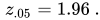
where $\ y_{\alpha }\$ is the lower $\ {\tfrac {\alpha }{2}}\$ quantile of a standard normal distribution, vs. $\ z_{\alpha }\ ,$ which is the upper ( i.e., $\ 1-{\tfrac {\alpha }{2}}\$ ) quantile.

Since the test in the middle of the inequality is a Wald test, the normal approximation interval is sometimes called the Wald interval or Wald method, after Abraham Wald, but it was first described by Laplace (1812).

02Standard error of a proportion estimation when using weighted data

To apply the principles of the weighted data correctly, you need to understand the type of the weight you are dealing with. For analytic weights, the following calculation can be applied.

Let $\ X_{1},\ \ldots ,\ X_{n}\$ be such that each $\ X_{i}\$ is i.i.d from a Bernoulli( p ) distribution and weight $\ w_{i}\$ is the weight for each observation, with the (positive) weights $\ w_{i}\$ normalized so they sum to 1 . The weighted sample proportion is: ${\textstyle \ {\hat {p}}=\sum _{i=1}^{n}w_{i}X_{i}~.$ Since each of the $\ X_{i}\$ is independent from all the others, and each one has variance $\ \operatorname {var} \{\ X_{i}\ \}=p\left(1-p\right)\$ for every $\ i=1,\ \ldots ,\ n\ ;$ the sampling variance of the proportion therefore is:

$\operatorname {var} \left\{\ {\hat {p}}\ \right\}~=~\sum _{i=1}^{n}\operatorname {var} \left\{\ w_{i}X_{i}\ \right\}~=~p\left(1-p\right)\sum _{i=1}^{n}w_{i}^{2}~.$

The standard error of $\ {\hat {p}}\$ is the square root of this quantity. Because we do not know $\ p\left(1-p\right)\ ,$ we have to estimate it. Although there are many possible estimators, a conventional one is to use $\ {\hat {p}}\ ,$ the sample mean, and plug this into the formula. That gives:

$\operatorname {SE} \left\{\ {\hat {p}}\ \right\}~\approx ~{\sqrt {{\hat {p}}\left(1-{\hat {p}}\right)\sum _{i=1}^{n}w_{i}^{2}~}}~.$

For otherwise unweighted data, the effective weights are uniform ${\textstyle \ w_{i}={\frac {1}{n}}\ ,$ giving ${\textstyle \ \sum _{i=1}^{n}w_{i}^{2}={\frac {1}{n}}~.$ The $\ \operatorname {SE} \$ becomes ${\textstyle \ {\sqrt {{\tfrac {1}{n}}\ {\hat {p}}\left(1-{\hat {p}}\right)\ }}\ ,$ leading to the familiar formulas, showing that the calculation for weighted data is a direct generalization of them.

If the weights in question are the complex sampling design weights, appropriate statistical software (R package survey; Python package svy) needs to be used to obtain standard errors corrected for the survey sampling design. An extension of the § Clopper-Pearson interval presented below to the complex survey data is also known as the Korn-Graubard confidence interval.

03Wilson score interval

The Wilson score interval was developed by E.B. Wilson (1927). It is an improvement over the normal approximation interval in multiple respects: Unlike the symmetric normal approximation interval (above), the Wilson score interval is asymmetric, and it doesn't suffer from problems of overshoot and zero-width intervals that afflict the normal interval. It can be safely employed with small samples and skewed observations. The observed coverage probability is consistently closer to the nominal value, $\ 1-\alpha ~.$ .

Like the normal interval, the interval can be computed directly from a formula.

Wilson started with the normal approximation to the binomial: $z_{\alpha }\ \approx \ {\frac {p-{\hat {p}}}{\sigma _{n}}}$ where $\ z_{\alpha }\$ is the standard normal interval half-width corresponding to the desired confidence $\ 1-\alpha ~.$ The analytic formula for a binomial sample standard deviation is $\sigma _{n}={\sqrt {\frac {p\left(1-p\right)}{n}}}~.$ Combining the two, and squaring out the radical, gives an equation that is quadratic in $\ p\ :$ $\left(p-{\hat {p}}\right)^{2}~=~{\frac {\ z_{\alpha }^{2}}{n}}\ p\left(1-p\right)$ or $p^{2}\ -\ 2\ p\ {\hat {p}}\ +\ {\hat {p}}^{2}~=~p\ {\frac {z_{\alpha }^{2}}{n}}\ -\ p^{2}\ {\frac {z_{\alpha }^{2}}{n}}~.$ Transforming the relation into a standard-form quadratic equation for $\ p\ ,$ treating $\ {\hat {p}}\$ and $\ n\$ as known values from the sample (see prior section), and using the value of $\ z_{\alpha }\$ that corresponds to the desired confidence $\ 1-\alpha \$ for the estimate of $\ p\$ gives this: $\left(1+{\frac {z_{\alpha }^{2}}{n}}\right)p^{2}-\left(2{\hat {p}}+{\frac {z_{\alpha }^{2}}{n}}\right)p+{\biggl (}\ {\hat {p}}^{2}{\biggr )}=0\ ,$ where all of the values bracketed by parentheses are known quantities. The solution for $\ p\$ estimates the upper and lower limits of the confidence interval for $\ p~.$ Hence the probability of success $\ p\$ is estimated by $\ {\hat {p}}\$ and with $\ 1-\alpha \$ confidence bracketed in the interval $p~~{\underset {\approx }{\in }}_{\alpha }\;\left(\ w^{-},w^{+}\ \right)~=~{\frac {1}{1+z_{\alpha }^{2}/n}}\left(\ {\hat {p}}+{\frac {z_{\alpha }^{2}}{2\ n}}\ \pm \ {\frac {z_{\alpha }}{2\ n}}{\sqrt {4\ n\ {\hat {p}}\left(1-{\hat {p}}\right)+z_{\alpha }^{2}\ }}\ \right)$

where $\ {\underset {\approx }{\in }}_{\alpha }\$ is an abbreviation for

$\operatorname {\mathbb {P} } \left\{\ p\in \left(w^{-},w^{+}\right)\ \right\}=1-\alpha ~.$

An equivalent expression using the observation counts $\ n_{\mathsf {s}}\$ and $\ n_{\mathsf {f}}\$ is $p~~{\underset {\approx }{\in }}_{\alpha }\;{\frac {\ n_{\mathsf {s}}+{\tfrac {1}{2}}\ z_{\alpha }^{2}}{\ n+z_{\alpha }^{2}}}~\pm ~{\frac {\ z_{\alpha }}{~n+z_{\alpha }^{2}\ }}{\sqrt {{\frac {\ n_{\mathsf {s}}\ n_{\mathsf {f}}}{n}}+{\frac {\ z_{\alpha }^{2}}{4}}~}}\ ,$

with the counts as above: $\ n_{\mathsf {s}}\equiv$ the count of observed "successes", $\ n_{\mathsf {f}}\equiv$ the count of observed "failures", and their sum is the total number of observations $\ n=n_{\mathsf {s}}+n_{\mathsf {f}}~.$

In practical tests of the formula's results, users find that this interval has good properties even for a small number of trials and / or the extremes of the probability estimate, $\ {\hat {p}}\equiv {\frac {n_{\mathsf {s}}}{n}}~.$

Intuitively, the center value of this interval is the weighted average of $\ {\hat {p}}\$ and ${\textstyle \ {\tfrac {1}{2}}\ ,$ with $\ {\hat {p}}\$ receiving greater weight as the sample size increases. Formally, the center value corresponds to using a pseudocount of $\ {\tfrac {1}{2}}z_{\alpha }^{2}\ ,$ the number of standard deviations of the confidence interval: Add this number to both the count of successes and of failures to yield the estimate of the ratio. For the common two standard deviations in each direction interval (approximately 95% coverage, which itself is approximately 1.96 standard deviations), this yields the estimate $\ {\frac {n_{\mathsf {s}}+2}{n+4}}\ ,$ which is known as the "plus four rule".

Although the quadratic can be solved explicitly, in most cases Wilson's equations can also be solved numerically using the fixed-point iteration $p_{k+1}={\hat {p}}\pm z_{\alpha }{\sqrt {{\tfrac {1}{n}}p_{k}\left(1-p_{k}\right)~}}$ with $\ p_{0}={\hat {p}}~.$

The Wilson interval can also be derived from the single sample z-test or Pearson's chi-squared test with two categories. The resulting interval,

$\left\{~\theta \quad {\Bigg |}\quad y_{\alpha }~~\leq ~~{\frac {{\hat {p}}-\theta }{\sqrt {{\tfrac {\!1\!}{n}}\theta \left(1-\theta \right)~}}}~~\leq ~~z_{\alpha }~\right\}\ ,$

(with $y_{\alpha }$ the lower $\alpha$ quantile) can then be solved for $\theta$ to produce the Wilson score interval. The test in the middle of the inequality is a score test.

The interval equality principle

Since the interval is derived by solving from the normal approximation to the binomial, the Wilson score interval $\ \left(w^{-},w^{+}\right)\$ has the property of being guaranteed to obtain the same result as the equivalent z-test or chi-squared test.

This property can be visualised by plotting the probability density function for the Wilson score interval (see Wallis). After that, then also plotting a normal pdf across each bound. The tail areas of the resulting Wilson and normal distributions represent the chance of a significant result, in that direction, must be equal.

The continuity-corrected Wilson score interval and the Clopper-Pearson interval are also compliant with this property. The practical import is that these intervals may be employed as significance tests, with identical results to the source test, and new tests may be derived by geometry.

Wilson score interval with continuity correction

The Wilson interval may be modified by employing a continuity correction, in order to align the minimum coverage probability, rather than the average coverage probability, with the nominal value, $\ 1-\alpha ~.$

Just as the Wilson interval mirrors Pearson's chi-squared test, the Wilson interval with continuity correction mirrors the equivalent Yates' chi-squared test.

The following formulae for the lower and upper bounds of the Wilson score interval with continuity correction $\ \left(w_{\mathsf {cc}}^{-},w_{\mathsf {cc}}^{+}\right)\$ are derived from Newcombe: ${\begin{aligned}w_{\mathsf {cc}}^{-}&=\max \left\{~0,~{\frac {2n{\hat {p}}+z_{\alpha }^{2}-\left[z_{\alpha }{\sqrt {z_{\alpha }^{2}-{\frac {1}{n}}+4n{\hat {p}}\left(1-{\hat {p}}\right)+\left(4{\hat {p}}-2\right)~}}+1\right]}{2\left(n+z_{\alpha }^{2}\right)~}}\right\}\ ,\\w_{\mathsf {cc}}^{+}&=\min \left\{~~1,~~{\frac {2n{\hat {p}}+z_{\alpha }^{2}+\left[z_{\alpha }{\sqrt {z_{\alpha }^{2}-{\frac {1}{n}}+4n{\hat {p}}\left(1-{\hat {p}}\right)-\left(4{\hat {p}}-2\right)~}}+1\right]}{2\left(n+z_{\alpha }^{2}\right)~~}}\right\}\ ,\end{aligned}}$ for $\ {\hat {p}}\neq 0\$ and $\ {\hat {p}}\neq 1~.$

If $\ {\hat {p}}=0\ ,$ then $\ w_{\mathsf {cc}}^{-}\$ must instead be set to $\ 0\ ;$ if $\ {\hat {p}}=1\ ,$ then $\ w_{\mathsf {cc}}^{+}\$ must be instead set to $\ 1~.$

Wallis (2026) identifies a simpler method for computing continuity-corrected Wilson intervals that employs a special function based on Wilson's formula: In Wallis' notation, for the lower bound, let ${\mathsf {Wilson_{lower}}}\!\left(\ {\hat {p}},\ n,\ \alpha \right)~\equiv ~w^{-}~=~{\frac {1}{~1+z_{\alpha }^{2}/n~}}{\Biggl (}\ {\hat {p}}+{\frac {\;z_{\alpha }^{2}}{2n}}~~-~~{\frac {\ z_{\alpha }}{2n}}{\sqrt {4n{\hat {p}}(1-{\hat {p}})+z_{\alpha }^{2}~}}~{\Biggr )}\ ,$ where $\ \alpha \$ is the selected tolerable error level for $\ z_{\alpha }$ . The upper bound, ${\mathsf {Wilson_{upper}}}$ is obtained from ${\mathsf {Wilson_{upper}}}\!\left(\ {\hat {p}},\ n,\ \alpha \right)~\equiv ~w^{+}~=~{\frac {1}{~1+z_{\alpha }^{2}/n~}}{\Biggl (}\ {\hat {p}}+{\frac {\;z_{\alpha }^{2}}{2n}}~~+~~{\frac {\ z_{\alpha }}{2n}}{\sqrt {4n{\hat {p}}(1-{\hat {p}})+z_{\alpha }^{2}~}}~{\Biggr )}\ .$ Then $w_{\mathsf {cc}}^{-}~=~{\mathsf {Wilson_{lower}}}\!\left(\ \max \left\{\ {\hat {p}}-{\tfrac {1}{2n}},\ 0\ \right\},\ n,~~\alpha \right)~,$ and $w_{\mathsf {cc}}^{+}~=~{\mathsf {Wilson_{upper}}}\!\left(\ \min \left\{\ {\hat {p}}+{\tfrac {1}{2n}},\ 1\ \right\},\ n,~~\alpha \right)~.$ This method has the advantage of being further decomposable.

To apply a continuity correction to the Wilson interval with such an adjusted ${\tilde {n}}$ , we modify the second parameter of Wallis' Wilson formulae above, but leave the continuity adjustment term ${\tfrac {1}{2n}}$ unaltered (Wallis 2026).

Wilson interval with complex survey data

For complex survey data, such as when sampling from a finite population, or sampling with unequal weighting and clustering, the sample size $n$ needs to be replaced with the effective sample size ${\tilde {n}}=n/{\rm {DEFF}}$ that accounts for the design effect of sampling.

It may also be reasonable to replace the normal quantiles $z_{\alpha }$ with the Student distribution quantiles $t_{\alpha }(d)$ where $d$ is the sampling design degrees of freedom.

04Jeffreys interval

The Jeffreys interval has a Bayesian derivation, but good frequentist properties (outperforming most frequentist constructions). In particular, it has coverage properties that are similar to those of the Wilson interval, but it is one of the few intervals with the advantage of being equal-tailed (e.g., for a 95% confidence interval, the probabilities of the interval lying above or below the true value are both close to 2.5%). In contrast, the Wilson interval has a systematic bias such that it is centred too close to $p=0.5$ .

The Jeffreys interval is the Bayesian credible interval obtained when using the non-informative Jeffreys prior for the binomial proportion $p~.$ The Jeffreys prior for this problem is a Beta distribution with parameters $\left({\tfrac {\!1\!}{2}},{\tfrac {\!1\!}{2}}\right),$ a conjugate prior. After observing $x$ successes in $n$ trials, the posterior distribution for $p$ is a Beta distribution with parameters $\left(x+{\tfrac {\!1\!}{2}},n-x+{\tfrac {\!1\!}{2}}\right)~.$

When $x\neq 0$ and $x\neq n,$ the Jeffreys interval is taken to be the $100\left(1-\alpha \right)\mathrm {\%}$ equal-tailed posterior probability interval, i.e., the ${\tfrac {\!1\!}{2}}\alpha$ and $1-{\tfrac {\!1\!}{2}}\alpha$ quantiles of a Beta distribution with parameters $\left(x+{\tfrac {1}{2}},n-x+{\tfrac {1}{2}}\right)~.$

In order to avoid the coverage probability tending to zero when $p\to 0$ or 1 , when $x=0$ the upper limit is calculated as before but the lower limit is set to 0 , and when $x=n$ the lower limit is calculated as before but the upper limit is set to 1 .

Jeffreys' interval can also be thought of as a frequentist interval based on inverting the p-value from the G-test after applying the Yates correction to avoid a potentially-infinite value for the test statistic.

05Clopper-Pearson interval

The Clopper-Pearson interval is an early and very common method for calculating binomial confidence intervals. This is often called an 'exact' method, as it attains the nominal coverage level in an exact sense, meaning that the coverage level is never less than the nominal $1-\alpha$ .

The Clopper-Pearson interval can be written as

$S_{\leq }\cap S_{\geq }$

or equivalently,

$\left(\inf S_{\geq },\sup S_{\leq }\right)$

with

$S_{\leq }~\equiv ~\left\{~p~{\Big |}~\operatorname {\mathbb {P} } \left\{~\operatorname {Bin} \left(n;p\right)\leq x\right\}>{\tfrac {\alpha }{2}}~\right\}~$ and $S_{\geq }~\equiv ~\left\{~p~{\Big |}~\operatorname {\mathbb {P} } \left\{~\operatorname {Bin} \left(n;p\right)\geq x\right\}>{\tfrac {\alpha }{2}}~\right\},$

where $0\leq x\leq n$ is the number of successes observed in the sample and ${\mathsf {Bin}}\left(n;p\right)$ is a binomial random variable with $n$ trials and probability of success $p~.$

Equivalently we can say that the Clopper-Pearson interval is ${\textstyle \left({\frac {\!x\!}{n}}-\varepsilon _{1},{\frac {\!x\!}{n}}+\varepsilon _{2}\right)$ with confidence level $1-\alpha$ if $\varepsilon _{i}$ is the infimum of those such that the following tests of hypothesis succeed with significance ${\textstyle {\frac {\!\alpha \!}{2}}:$

H₀: $p={\frac {\!x\!}{n}}-\varepsilon _{1}$ with H_A: $p>{\frac {\!x\!}{n}}-\varepsilon _{1}$
H₀: $p={\frac {\!x\!}{n}}+\varepsilon _{2}$ with H_A: $p<{\frac {\!x\!}{n}}+\varepsilon _{2}~.$

Because of a relationship between the binomial distribution and the beta distribution, the Clopper-Pearson interval is sometimes presented in an alternate format that uses quantiles from the beta distribution.

$B\!\left({\tfrac {\!\alpha \!}{2}};x,n-x+1\right)~<~p~<~B\!\left(1-{\tfrac {\!\alpha \!}{2}};x+1,n-x\right)$

where $x$ is the number of successes, $n$ is the number of trials, and $B\!\left(p;v,w\right)$ is the pth quantile from a beta distribution with shape parameters $v$ and $w~.$

Thus, $p_{\min }~<~p<~p_{\max },$ where: ${\tfrac {\Gamma (n+1)}{\Gamma \!(x)\Gamma \!(n-x+1)}}\int _{0}^{p_{\min }}t^{x-1}(1-t)^{n-x}\mathrm {d} \!t~~=~~{\tfrac {\!\alpha \!}{2}},$ ${\tfrac {\Gamma (n+1)}{\Gamma (x+1)\Gamma (n-x)}}\int _{0}^{p_{\max }}t^{x}(1-t)^{n-x-1}\mathrm {d} \!t~=~1-{\tfrac {\!\alpha \!}{2}}~.$ The binomial proportion confidence interval is then $\left(p_{\min },p_{\max }\right),$ as follows from the relation between the Binomial distribution cumulative distribution function and the regularized incomplete beta function.

When $x$ is either 0 or $n,$ closed-form expressions for the interval bounds are available: when $x=0$ the interval is ${\textstyle \left(0,1-\left({\tfrac {\!\alpha \!}{2}}\right)^{1/n}\right)$ and when $x=n$ it is ${\textstyle \left(\left({\tfrac {\!\alpha \!}{2}}\right)^{1/n},1\right)~.$

The beta distribution is, in turn, related to the F-distribution so a third formulation of the Clopper-Pearson interval can be written using F quantiles:

$\left(1+{\frac {n-x+1}{xF\!\left[{\tfrac {\alpha }{2}};2x,2(n-x+1)\right]}}\right)^{-1}~<~p~<~\left(1+{\frac {n-x}{(x+1)F\!\left[1-{\tfrac {\alpha }{2}};2(x+1),2(n-x)\right]}}\right)^{-1}$

where $x$ is the number of successes, $n$ is the number of trials, and $F\!\left(c;d_{1},d_{2}\right)$ is the $c$ quantile from an F-distribution with $d_{1}$ and $d_{2}$ degrees of freedom.

The Clopper-Pearson interval is an 'exact' interval, since it is based directly on the binomial distribution rather than any approximation to the binomial distribution. This interval never has less than the nominal coverage for any population proportion, but that means that it is usually conservative. For example, the true coverage rate of a 95% Clopper-Pearson interval may be well above 95%, depending on $n$ and $p~.$ Thus the interval may be wider than it needs to be to achieve 95% confidence, and wider than other intervals. In contrast, it is worth noting that other confidence interval may have coverage levels that are lower than the nominal $1-\alpha ,$ i.e., the normal approximation (or "standard") interval, Wilson interval, Agresti-Coull interval, etc., with a nominal coverage of 95% may in fact cover less than 95%, even for large sample sizes.

The definition of the Clopper-Pearson interval can also be modified to obtain exact confidence intervals for different distributions. For instance, it can also be applied to the case where the samples are drawn without replacement from a population of a known size, instead of repeated draws of a binomial distribution. In this case, the underlying distribution would be the hypergeometric distribution.

The interval boundaries can be computed with numerical functions qbeta in R and scipy.stats.beta.ppf in Python.

from scipy.stats import beta import numpy as np k = 20 n = 400 alpha = 0.05 p_u, p_o = beta.ppf([alpha / 2, 1 - alpha / 2], [k, k + 1], [n - k + 1, n - k]) if np.isnan(p_o): p_o = 1 if np.isnan(p_u): p_u = 0

06Agresti-Coull interval

The Agresti-Coull interval is also another approximate binomial confidence interval.

Given $n_{\mathsf {s}}$ successes in $n$ trials, define ${\tilde {n}}\equiv n+z_{\alpha }^{2}$

and ${\tilde {p}}={\frac {1}{\tilde {n}}}\left(\!n_{\mathsf {s}}+{\tfrac {z_{\alpha }^{2}}{2}}\!\right)$

Then, a confidence interval for $p$ is given by

$p~~\approx ~~{\tilde {p}}~\pm ~z_{\alpha }{\sqrt {{\frac {\!{\tilde {p}}\!}{\tilde {n}}}\left(\!1-{\tilde {p}}\!\right)~}}$

where $z_{\alpha }=\operatorname {\Phi ^{-1}} \!\!\left(1-{\tfrac {\!\alpha \!}{2}}\right)$ is the quantile of a standard normal distribution, as before (for example, a 95% confidence interval requires $\alpha =0.05,$ thereby producing $z_{.05}=1.96$ ). According to Brown, Cai, & DasGupta (2001), taking $z=2$ instead of 1.96 produces the "add 2 successes and 2 failures" interval previously described by Agresti & Coull.

This interval can be summarised as employing the centre-point adjustment, ${\tilde {p}},$ of the Wilson score interval, and then applying the Normal approximation to this point.

${\tilde {p}}={\frac {\quad {\hat {p}}+{\frac {z_{\alpha }^{2}\!}{2n}}\quad }{\quad 1+{\frac {z_{\alpha }^{2}}{n}}\quad }}$

07Arcsine transformation

The arcsine transformation has the effect of pulling out the ends of the distribution. While it can stabilize the variance (and thus confidence intervals) of proportion data, its use has been criticized in several contexts.

Let $X$ be the number of successes in $n$ trials and let $p={\tfrac {1}{\!n\!}}\!X~.$ The variance of $p$ is

$\operatorname {var} \{~~p~~\}={\tfrac {1}{\!n\!}}p(1-p)~.$

Using the arc sine transform, the variance of the arcsine of ${\sqrt {p~}}$ is

$\operatorname {var} \left\{~~\arcsin {\sqrt {p~}}~~\right\}~\approx ~{\frac {\operatorname {var} \{~~p~~\}}{4p(1-p)}}={\frac {p(1-p)}{4np(1-p)}}={\frac {1}{4n}}~.$

So, the confidence interval itself has the form

$\sin ^{2}\left(-{\frac {z_{\alpha }}{2{\sqrt {n}}}}+\arcsin {\sqrt {p}}~\right)~<~\theta ~<~\sin ^{2}\left(+{\frac {z_{\alpha }}{2{\sqrt {n}}}}+\arcsin {\sqrt {p}}~\right),$

where $z_{\alpha }$ is the $1-{\tfrac {\!\alpha \!}{2}}$ quantile of a standard normal distribution.

This method may be used to estimate the variance of $p$ but its use is problematic when $p$ is close to 0 or 1 .

08ta transform

Let $p$ be the proportion of successes. For $0\leq a\leq 2,$

$t_{a}=\log \left({\frac {p^{a}}{(1-p)^{2-a}}}\right)=a\log p-(2-a)\log(1-p)$

This family is a generalisation of the logit transform which is a special case with a = 1 and can be used to transform a proportional data distribution to an approximately normal distribution. The parameter a has to be estimated for the data set.

09Rule of three, for when no successes are observed

The rule of three is used to provide a simple way of stating an approximate 95% confidence interval for $p$ , in the special case that no successes ( ${\hat {p}}=0$ ) have been observed. The interval is $\left(0,{\tfrac {3}{n}}\right)$ .

By symmetry, in the case of only successes ( ${\hat {p}}=1$ ), the interval is $\left(1-{\tfrac {3}{n}},1\right)$ .

10Comparison and discussion

There are several research papers that compare these and other confidence intervals for the binomial proportion.

Both Ross (2003) and Agresti & Coull (1998) point out that exact methods such as the Clopper-Pearson interval may not work as well as some approximations. The normal approximation interval and its presentation in textbooks has been heavily criticised, with many statisticians advocating that it not be used. The principal problems are overshoot (bounds exceed [0, 1]), zero-width intervals at ${\hat {p}}=0$ or 1 (falsely implying certainty),, inaccurate coverage (the actual coverage is not equal to the nominal level such as 95%) and overall inconsistency with significance testing.

Of the approximations listed above, Wilson score interval methods (with or without continuity correction) have been shown to be the most accurate and the most robust, though some prefer Agresti & Coull's approach for larger sample sizes. Wilson and Clopper-Pearson methods obtain consistent results with source significance tests, and this property is decisive for many researchers.

Many of these intervals can be calculated in R using packages like binom and survey; and in Python using statsmodels function proportion_confint()

Watch videos about Binomial proportion confidence intervalExplainers and documentaries on YouTube (opens in a new tab)

Sources and credits

This article is adapted from the Wikipedia article “Binomial proportion confidence interval”, written by its contributors and licensed under CC BY-SA 4.0. Fathomly has changed the layout, removed citation markers, navigation and maintenance notices, and adjusted punctuation. This adapted version is shared under the same license. For references, see the original article.

Images, from Wikimedia Commons:

Wilson score pdf and interval equality.png by Unknown author, CC-BY-SA-4.0
Normal approx interval and logistic example.png by Unknown author, CC BY 4.0
Wilson score interval and logistic example.png by Unknown author, CC BY 4.0
Jeffreys intervals plotted on a logistic curve.svg by Iroqu, CC BY-SA 4.0

Fathomly is not affiliated with or endorsed by the Wikimedia Foundation. Spotted a problem? Tell us.