Encyclopedia

Population proportion

Parameters which denote fractions of populations, usually as a percentage

Wikipedia contributorsAdapted for Fathomly · View authors

5 min read
Source updated May 20, 2026

In statistics a population proportion, generally denoted by $P$ or the Greek letter $\pi$ , is a parameter that describes a percentage value associated with a population. A census can be conducted to determine the actual value of a population parameter, but often a census is not practical due to its costs and time consumption. For example, the 2010 United States census showed that 83.7% of the American population was identified as not being Hispanic or Latino; the value of .837 is a population proportion. In general, the population proportion and other population parameters are unknown.

A population proportion is usually estimated through an unbiased sample statistic obtained from an observational study or experiment, resulting in a sample proportion, generally denoted by ${\hat {p}}$ and in some textbooks by $p$ . For example, the National Technological Literacy Conference conducted a national survey of 2,000 adults to determine the percentage of adults who are economically illiterate; the study showed that 1,440 out of the 2,000 adults sampled did not understand what a gross domestic product is. The value of 72% (or 1440/2000) is a sample proportion.

01Mathematical definition

A proportion is mathematically defined as being the ratio of the quantity of elements (a countable quantity) in a subset $S$ to the size of a set $R$ :

$P={\frac {X}{N}},$

where $X$ is the count of successes in the population, and $N$ is the size of the population.

This mathematical definition can be generalized to provide the definition for the sample proportion:

${\hat {p}}={\frac {x}{n}}$

where $x$ is the count of successes in the sample, and $n$ is the size of the sample obtained from the population.

A Venn Diagram illustration of a set and its subset . The proportion can be calculated by measuring how much of is in .

02Estimation

One of the main focuses of study in inferential statistics is determining the "true" value of a parameter. Generally the actual value for a parameter will never be found, unless a census is conducted on the population of study. However, there are statistical methods that can be used to get a reasonable estimation for a parameter. These methods include confidence intervals and hypothesis testing.

Estimating the value of a population proportion can be of great implication in the areas of agriculture, business, economics, education, engineering, environmental studies, medicine, law, political science, psychology, and sociology.

A population proportion can be estimated through the usage of a confidence interval known as a one-sample proportion in the Z-interval whose formula is given below:

${\hat {p}}\pm z^{*}{\sqrt {\frac {{\hat {p}}(1-{\hat {p}})}{n}}}$

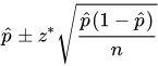
where ${\hat {p}}$ is the sample proportion, $n$ is the sample size, and $z^{*}$ is the upper ${\frac {1-C}{2}}$ critical value of the standard normal distribution for a level of confidence $C$ .

Proof

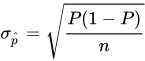
To derive the formula for the one-sample proportion in the Z-interval, a sampling distribution of sample proportions needs to be taken into consideration. The mean of the sampling distribution of sample proportions is usually denoted as $\mu _{\hat {p}}=P$ and its standard deviation is denoted as:

$\sigma _{\hat {p}}={\sqrt {\frac {P(1-P)}{n}}}$

Since the value of $P$ is unknown, an unbiased statistic ${\hat {p}}$ will be used for $P$ . The mean and standard deviation are rewritten respectively as:

$\mu _{\hat {p}}={\hat {p}}$ and $\sigma _{\hat {p}}={\sqrt {\frac {{\hat {p}}(1-{\hat {p}})}{n}}}$

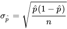
Invoking the central limit theorem, the sampling distribution of sample proportions is approximately normal, provided that the sample is reasonably large and unskewed.

Suppose the following probability is calculated:

$P\left(-z^{*}<{\frac {{\hat {p}}-P}{\sqrt {\frac {{\hat {p}}(1-{\hat {p}})}{n}}}}<z^{*}\right)=C$ ,

where $0<C<1$ and $\pm z^{*}$ are the standard critical values.

The inequality

$-z^{*}<{\frac {{\hat {p}}-P}{\sqrt {\frac {{\hat {p}}(1-{\hat {p}})}{n}}}}<z^{*}$

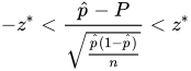
can be algebraically re-written as follows:

$-z^{*}<{\frac {{\hat {p}}-P}{\sqrt {\frac {{\hat {p}}(1-{\hat {p}})}{n}}}}<z^{*}$

$\Rightarrow -z^{*}{\sqrt {\frac {{\hat {p}}(1-{\hat {p}})}{n}}}<{\hat {p}}-P<z^{*}{\sqrt {\frac {{\hat {p}}(1-{\hat {p}})}{n}}}$

$\Rightarrow -{\hat {p}}-z^{*}{\sqrt {\frac {{\hat {p}}(1-{\hat {p}})}{n}}}<-P<-{\hat {p}}+z^{*}{\sqrt {\frac {{\hat {p}}(1-{\hat {p}})}{n}}}$

$\Rightarrow {\hat {p}}-z^{*}{\sqrt {\frac {{\hat {p}}(1-{\hat {p}})}{n}}}<P<{\hat {p}}+z^{*}{\sqrt {\frac {{\hat {p}}(1-{\hat {p}})}{n}}}$

Conditions for inference

In general the formula used for estimating a population proportion requires substitutions of known numerical values. However, these numerical values cannot be "blindly" substituted into the formula because statistical inference requires that the estimation of an unknown parameter be justifiable. For a parameter's estimation to be justifiable, there are three conditions that need to be verified:

The data's individual observation have to be obtained from a simple random sample of the population of interest.
The data's individual observations have to display normality. This can be assumed mathematically with the following definition:
- Let $n$ be the sample size of a given random sample and let ${\hat {p}}$ be its sample proportion. If $n{\hat {p}}\geq 10$ and $n(1-{\hat {p}})\geq 10$ , then the data's individual observations display normality.
The data's individual observations have to be independent of each other. This can be assumed mathematically with the following definition:
- Let $N$ be the size of the population of interest and let $n$ be the sample size of a simple random sample of the population. If $N\geq 10n$ , then the data's individual observations are independent of each other.

The conditions for SRS, normality, and independence are sometimes referred to as the conditions for the inference tool box in most statistical textbooks.

Example

Suppose a presidential election is taking place in a democracy. A random sample of 400 eligible voters in the democracy's voter population shows that 272 voters support candidate B. A political scientist wants to determine what percentage of the voter population support candidate B.

To answer the political scientist's question, a one-sample proportion in the Z-interval with a confidence level of 95% can be constructed in order to determine the population proportion of eligible voters in this democracy that support candidate B.

Solution

It is known from the random sample that 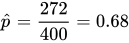${\hat {p}}={\frac {272}{400}}=0.68$ with sample size $n=400$ . Before a confidence interval is constructed, the conditions for inference will be verified.

Since a random sample of 400 voters was obtained from the voting population, the condition for a simple random sample has been met.
Let $n=400$ and ${\hat {p}}=0.68$ , it will be checked whether $n{\hat {p}}\geq 10$ and $n(1-{\hat {p}})\geq 10$

$(400)(0.68)\geq 10\Rightarrow 272\geq 10$ and $(400)(1-0.68)\geq 10\Rightarrow 128\geq 10$

The condition for normality has been met.

Let $N$ be the size of the voter population in this democracy, and let $n=400$ . If $N\geq 10n$ , then there is independence.

$N\geq 10(400)\Rightarrow N\geq 4000$

The population size $N$ for this democracy's voters can be assumed to be at least 4,000. Hence, the condition for independence has been met.

With the conditions for inference verified, it is permissible to construct a confidence interval.

Let ${\hat {p}}=0.68,n=400,$ and $C=0.95$

To solve for $z^{*}$ , the expression ${\frac {1-C}{2}}$ is used.

${\frac {1-C}{2}}={\frac {1-0.95}{2}}={\frac {0.05}{2}}=0.0250$

By examining a standard normal bell curve, the value for $z^{*}$ can be determined by identifying which standard score gives the standard normal curve an upper tail area of 0.0250 or an area of 1, 0.0250 = 0.9750. The value for $z^{*}$ can also be found through a table of standard normal probabilities.

From a table of standard normal probabilities, the value of $Z$ that gives an area of 0.9750 is 1.96. Hence, the value for $z^{*}$ is 1.96.

The values for ${\hat {p}}=0.68$ , $n=400$ , $z^{*}=1.96$ can now be substituted into the formula for one-sample proportion in the Z-interval:

${\hat {p}}\pm z^{*}{\sqrt {\frac {{\hat {p}}(1-{\hat {p}})}{n}}}$

$\Rightarrow (0.68)\pm (1.96){\sqrt {\frac {(0.68)(1-0.68)}{400}}}$

$\Rightarrow 0.68\pm 1.96{\sqrt {0.000544}}$

$\Rightarrow {\bigl (}0.63429,\,0.72571{\bigr )}$

Based on the conditions of inference and the formula for the one-sample proportion in the Z-interval, it can be concluded with a 95% confidence level that the percentage of the voter population in this democracy supporting candidate B is between 63.429% and 72.571%.

Value of the parameter in the confidence interval range

A commonly asked question in inferential statistics is whether the parameter is included within a confidence interval. The only way to answer this question is for a census to be conducted. Referring to the example given above, the probability that the population proportion is in the range of the confidence interval is either 1 or 0. That is, the parameter is included in the interval range or it is not. The main purpose of a confidence interval is to better illustrate what the ideal value for a parameter could possibly be.

Common errors and misinterpretations from estimation

A very common error that arises from the construction of a confidence interval is the belief that the level of confidence, such as $C=95\%$ , means 95% chance. This is incorrect. The level of confidence is based on a measure of certainty, not probability. Hence, the values of $C$ fall between 0 and 1, exclusively.

Estimation of P using ranked set sampling

A more precise estimate of P can be obtained by choosing ranked set sampling instead of simple random sampling

Watch videos about Population proportionExplainers and documentaries on YouTube (opens in a new tab)

Sources and credits

This article is adapted from the Wikipedia article “Population proportion”, written by its contributors and licensed under CC BY-SA 4.0. Fathomly has changed the layout, removed citation markers, navigation and maintenance notices, and adjusted punctuation. This adapted version is shared under the same license. For references, see the original article.

Images, from Wikimedia Commons:

SubsetMine.png by LawrenceSeminarioRomero, CC BY-SA 4.0
Sampling Distribution of Sample Proportions Edited.png by LawrenceSeminarioRomero, CC BY-SA 4.0
BELL CURVE.png by LawrenceSeminarioRomero, CC BY-SA 4.0
Table of Standard Normal Probabilities.png by LawrenceSeminarioRomero, CC BY-SA 4.0

Fathomly is not affiliated with or endorsed by the Wikimedia Foundation. Spotted a problem? Tell us.