Encyclopedia

Vapnik-Chervonenkis dimension

Notion in supervised machine learning

Wikipedia contributorsAdapted for Fathomly · View authors

8 min read
Source updated June 30, 2026

In Vapnik-Chervonenkis theory, the Vapnik-Chervonenkis (VC) dimension is a measure of the size (capacity, complexity, expressive power, richness, or flexibility) of a class of sets. The notion can be extended to classes of binary functions. It is defined as the cardinality of the largest set of points that the function class can shatter, that is, for which all possible binary labelings can be realized by some function in the class. It was originally defined by Vladimir Vapnik and Alexey Chervonenkis.

Informally, the capacity of a classification model is related to how complicated it can be. For example, consider the thresholding of a high-degree polynomial: if the polynomial evaluates above zero, that point is classified as positive, otherwise as negative. A high-degree polynomial can be wiggly, so that it can fit a given set of training points well. Such a polynomial has a high capacity. A much simpler alternative is to threshold a linear function. This function may not fit the training set well, because it has a low capacity. This notion of capacity is made rigorous below.

01Definitions

VC dimension of a set-family

Let ${\mathcal {C}}=\{C\}_{C\in {\mathcal {C}}}$ be a family of sets (also called set family, collection of sets, or set of sets) and $X$ be a set. Their intersection is defined as the following set family:

${\mathcal {C}}\cap X:=\{C\cap X\mid C\in {\mathcal {C}}\}.$

Here typically $X$ and each $C\in {\mathcal {C}}$ are subsets of a big "universe" of possibilities $U$ where intersection takes place.

We say that a set $X$ is shattered by ${\mathcal {C}}$ if ${\mathcal {P}}(X)={\mathcal {C}}\cap X$ i.e. the set of intersections contains (hence is equal to the set of) all the subsets of $X$ . For finite sets $X$ this is equivalent to

$|{\mathcal {C}}\cap X|=2^{|X|}.$

The VC dimension $D$ of ${\mathcal {C}}$ is the cardinality of the largest set that is shattered by ${\mathcal {C}}$ . If arbitrarily large sets can be shattered, the VC dimension of ${\mathcal {C}}$ is $\infty$ .

VC dimension of a classification model

Consider a binary classification model $f$ with some parameter vector $\theta$ , a set of generally positioned data points $x_{1},x_{2},\ldots ,x_{n}$ . We say that the model $f$ shatters $x_{1},x_{2},\ldots ,x_{n}$ if, for every assignment of labels to those points, there exists a vector $\theta$ such that the model $f$ makes no errors when evaluating that set of data points.

The VC dimension of a model $f$ is the maximum number of points that can be arranged so that $f$ shatters them. More formally, it is the maximum cardinal $D$ such that there exists a generally positioned data point set of cardinality $D$ that can be shattered by $f$ .

02Examples

$f$ is a constant classifier (with no parameters); Its VC dimension is 0 since it cannot shatter even a single point. In general, the VC dimension of a finite classification model, which can return at most $2^{d}$ different classifiers, is at most $d$ (this is an upper bound on the VC dimension; the Sauer-Shelah lemma gives a lower bound on the dimension).
$f$ is a single-parametric threshold classifier on real numbers; i.e., for a certain threshold $\theta$ , the classifier $f_{\theta }$ returns 1 if the input number is larger than $\theta$ and 0 otherwise. The VC dimension of $f$ is 1 because: (a) It can shatter a single point. For every point $x$ , a classifier $f_{\theta }$ labels it as 0 if $\theta >x$ and labels it as 1 if $\theta <x$ . (b) It cannot shatter all the sets with two points. For every set of two numbers, if the smaller is labeled 1, then the larger must also be labeled 1, so not all labelings are possible.
$f$ is a single-parametric interval classifier on real numbers; i.e., for a certain parameter $\theta$ , the classifier $f_{\theta }$ returns 1 if the input number is in the interval $[\theta ,\theta +4]$ and 0 otherwise. The VC dimension of $f$ is 2 because: (a) It can shatter some sets of two points. E.g., for every set $\{x,x+2\}$ , a classifier $f_{\theta }$ labels it as (0,0) if $\theta <x-4$ or if $\theta >x+2$ , as (1,0) if $\theta \in [x-4,x-2)$ , as (1,1) if $\theta \in [x-2,x]$ , and as (0,1) if $\theta \in (x,x+2]$ . (b) It cannot shatter any set of three points. For every set of three numbers, if the smallest and the largest are labeled 1, then the middle one must also be labeled 1, so not all labelings are possible.
$f$ is a straight line as a classification model on points in a two-dimensional plane (this is the model used by a perceptron). The line should separate positive data points from negative data points. There exist sets of 3 points that can indeed be shattered using this model (any 3 points that are not collinear can be shattered). However, no set of 4 points can be shattered: by Radon's theorem, any four points can be partitioned into two subsets with intersecting convex hulls, so it is not possible to separate one of these two subsets from the other. Thus, the VC dimension of this particular classifier is 3. It is important to remember that while one can choose any arrangement of points, the arrangement of those points cannot change when attempting to shatter for some label assignment. Note, only 3 of the 2³ = 8 possible label assignments are shown for the three points.
$f$ is a single-parametric sine classifier, i.e., for a certain parameter $\theta$ , the classifier $f_{\theta }$ returns 1 if the input number $x$ has $\sin(\theta x)>0$ and 0 otherwise. The VC dimension of $f$ is infinite, since it can shatter any finite subset of the set $\{2^{-m}\mid m\in \mathbb {N} \}$ .


3 points shattered			4 points impossible

03Uses

In statistical learning theory

The VC dimension can predict a probabilistic upper bound on the test error of a classification model. Vapnik proved that the probability of the test error (i.e., risk with 0-1 loss function) distancing from an upper bound (on data that is drawn i.i.d. from the same distribution as the training set) is given by:

$\Pr \left({\text{test error}}\leqslant {\text{training error}}+{\sqrt {{\frac {1}{N}}\left[D\left(\log \left({\tfrac {2N}{D}}\right)+1\right)-\log \left({\tfrac {\eta }{4}}\right)\right]}}\,\right)=1-\eta ,$

where $D$ is the VC dimension of the classification model, $0<\eta \leqslant 1$ , and $N$ is the size of the training set (restriction: this formula is valid when $D\ll N$ . When $D$ is larger, the test-error may be much higher than the training-error. This is due to overfitting).

The VC dimension also appears in sample-complexity bounds. A space of binary functions with VC dimension $D$ can be learned with:

$N=\Theta \left({\frac {D+\ln {1 \over \delta }}{\varepsilon ^{2}}}\right)$

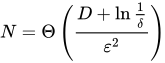
samples, where $\varepsilon$ is the learning error and $\delta$ is the failure probability. Thus, the sample-complexity is a linear function of the VC dimension of the hypothesis space.

In computational geometry

The VC dimension is one of the critical parameters in the size of ε-nets, which determines the complexity of approximation algorithms based on them; range sets without finite VC dimension may not have finite ε-nets at all.

04Bounds

The VC dimension of the dual set-family of ${\mathcal {C}}$ is strictly less than $2^{\operatorname {vc} ({\mathcal {C}})+1}$ , and this is best possible.
The VC dimension of a finite set-family ${\mathcal {C}}$ is at most $\log _{2}|{\mathcal {C}}|$ . This is because $|{\mathcal {C}}\cap X|\leq |X|$ by definition.
Given a set-family ${\mathcal {C}}$ , define ${\mathcal {C}}_{s}$ as a set-family that contains all intersections of $s$ elements of ${\mathcal {C}}$ . Then: $\operatorname {VCDim} ({\mathcal {C}}_{s})\leq \operatorname {VCDim} ({\mathcal {C}})\cdot (2s\log _{2}(3s))$
Given a set-family ${\mathcal {C}}$ and an element $C_{0}\in {\mathcal {C}}$ , define ${\mathcal {C}}\,\Delta C_{0}:=\{C\,\Delta C_{0}\mid C\in H\}$ where $\Delta$ denotes symmetric set difference. Then: $\operatorname {VCDim} ({\mathcal {C}}\,\Delta C_{0})=\operatorname {VCDim} ({\mathcal {C}})$

05Examples of VC Classes

VC dimension of a finite projective plane

A finite projective plane of order n is a collection of n² + n + 1 sets (called "lines") over n² + n + 1 elements (called "points"), for which:

Each line contains exactly n + 1 points.
Each line intersects every other line in exactly one point.
Each point is contained in exactly n + 1 lines.
Each point is in exactly one line in common with every other point.
At least four points do not lie in a common line.

The VC dimension of a finite projective plane is 2.

Proof: (a) For each pair of distinct points, there is one line that contains both of them, lines that contain only one of them, and lines that contain none of them, so every set of size 2 is shattered. (b) For any triple of three distinct points, if there is a line x that contain all three, then there is no line y that contains exactly two (since then x and y would intersect in two points, which is contrary to the definition of a projective plane). Hence, no set of size 3 is shattered.

VC dimension of a boosting classifier

Suppose we have a base class $B$ of simple classifiers, whose VC dimension is $D$ .

We can construct a more powerful classifier by combining several different classifiers from $B$ ; this technique is called boosting. Formally, given $T$ classifiers $h_{1},\ldots ,h_{T}\in B$ and a weight vector $w\in \mathbb {R} ^{T}$ , we can define the following classifier:

$f(x)=\operatorname {sign} \left(\sum _{t=1}^{T}w_{t}\cdot h_{t}(x)\right)$

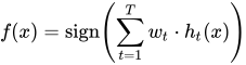
The VC dimension of the set of all such classifiers (for all selections of $T$ classifiers from $B$ and a weight-vector from $\mathbb {R} ^{T}$ ), assuming $T,D\geq 3$ , is at most:

$T\cdot (D+1)\cdot (3\log(T\cdot (D+1))+2)$

VC dimension of a neural network

A neural network is described by a directed acyclic graph G(V,E), where:

V is the set of nodes. Each node is a simple computation cell.
E is the set of edges, Each edge has a weight.
The input to the network is represented by the sources of the graph, the nodes with no incoming edges.
The output of the network is represented by the sinks of the graph, the nodes with no outgoing edges.
Each intermediate node gets as input a weighted sum of the outputs of the nodes at its incoming edges, where the weights are the weights on the edges.
Each intermediate node outputs a certain increasing function of its input, such as the sign function or the sigmoid function. This function is called the activation function.

The VC dimension of a neural network is bounded as follows:

If the activation function is the sign function and the weights are general, then the VC dimension is at most $O(|E|\cdot \log(|E|))$ .
If the activation function is the sigmoid function and the weights are general, then the VC dimension is at least $\Omega (|E|^{2})$ and at most $O(|E|^{2}\cdot |V|^{2})$ .
If the weights come from a finite family (e.g. the weights are real numbers that can be represented by at most 32 bits in a computer), then, for both activation functions, the VC dimension is at most $O(|E|)$ .

06Generalizations

The VC dimension is defined for spaces of binary functions (functions to {0,1}). Several generalizations have been suggested for spaces of non-binary functions.

For multi-class functions (e.g., functions to {0,...,n−1}), the Natarajan dimension, and its generalization the DS dimension can be used.
For real-valued functions (e.g., functions to a real interval, [0,1]), the Graph dimension or Pollard's pseudo-dimension can be used.
The Rademacher complexity provides similar bounds to the VC, and can sometimes provide more insight than VC dimension calculations into such statistical methods such as those using kernels.
The Memory Capacity (sometimes Memory Equivalent Capacity) gives a lower bound capacity, rather than an upper bound (see for example: Artificial neural network#Capacity) and therefore indicates the point of potential overfitting.

Watch videos about Vapnik-Chervonenkis dimensionExplainers and documentaries on YouTube (opens in a new tab)

Sources and credits

This article is adapted from the Wikipedia article “Vapnik-Chervonenkis dimension”, written by its contributors and licensed under CC BY-SA 4.0. Fathomly has changed the layout, removed citation markers, navigation and maintenance notices, and adjusted punctuation. This adapted version is shared under the same license. For references, see the original article.

Fathomly is not affiliated with or endorsed by the Wikimedia Foundation. Spotted a problem? Tell us.