Tukey lambda distribution
Symmetric probability distribution

Formalized by John Tukey, the Tukey lambda distribution is a continuous, symmetric probability distribution defined in terms of its quantile function. It is typically used to identify an appropriate distribution (see the comments below) and not used in statistical models directly.
The Tukey lambda distribution has a single shape parameter, λ, and as with other probability distributions, it can be transformed with a location parameter, μ, and a scale parameter, σ. Since the general form of probability distribution can be expressed in terms of the standard distribution, the subsequent formulas are given for the standard form of the function.
01Quantile function
For the standard form of the Tukey lambda distribution, the quantile function, 

![\ Q\left(\ p\ ;\lambda \ \right)~=~{\begin{cases}{\tfrac {1}{\ \lambda \ }}\left[\ p^{\lambda }-(1-p)^{\lambda }\ \right]\ ,&\ {\mbox{ if }}\ \lambda \neq 0~,\\{}\\\ln \left({\frac {p}{\ 1-p\ }}\right)~,&\ {\mbox{ if }}\ \lambda =0~.\end{cases}}](https://wikimedia.org/api/rest_v1/media/math/render/svg/9107f12b2e95f3e96724f02cd805d149cc8071cc)

For most values of the shape parameter, λ, the probability density function (PDF) and cumulative distribution function (CDF) must be computed numerically. The Tukey lambda distribution has a simple, closed form for the CDF and / or PDF only for a few exceptional values of the shape parameter, for example: λ ∈ { 2, 1, 1 /2, 0 } (see uniform distribution [ cases λ = 1 and λ = 2 ] and the logistic distribution [ case λ = 0 ].
However, for any value of λ both the CDF and PDF can be tabulated for any number of cumulative probabilities, p, using the quantile function Q to calculate the value x, for each cumulative probability p, with the probability density given by 1/q, the reciprocal of the quantile density function. As is the usual case with statistical distributions, the Tukey lambda distribution can readily be used by looking up values in a prepared table.
02Moments
The Tukey lambda distribution is symmetric around zero, therefore the expected value of this distribution, if it exists, is equal to zero. The variance exists for λ > − 1 /2 , and except when λ = 0 , is given by the formula
![\operatorname {Var} [\ X\ ]={\frac {2}{\lambda ^{2}}}{\bigg (}\ {\frac {1}{\ 1+2\lambda \ }}~-~{\frac {\ \Gamma (\lambda +1)^{2}\ }{\ \Gamma (2\lambda +2)\ }}\ {\bigg )}~.](https://wikimedia.org/api/rest_v1/media/math/render/svg/add74644e68e8440cbe473b57044b27e17692d44)
More generally, the n-th order moment is finite when λ > −1 /n and is expressed (except when λ = 0 ) in terms of the beta function Β(x,y) :
![\mu _{n}\equiv \operatorname {E} [\ X^{n}\ ]={\frac {1}{\lambda ^{n}}}\sum _{k=0}^{n}\ (-1)^{k}\ {n \choose k}\ \mathrm {B} (\ \lambda \ k+1\ ,\ (n-k)\ \lambda +1\ )~.](https://wikimedia.org/api/rest_v1/media/math/render/svg/18380dcd5031251e6db43228fc07e8f27993ad92)
Due to symmetry of the density function, all moments of odd orders, if they exist, are equal to zero.
03L-moments
Differently from the central moments, L-moments can be expressed in a closed form. For 


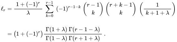
The first six L-moments can be presented as follows:

![\ell _{2}={\frac {2}{\ \lambda \ }}\ \left[\ -{\frac {1}{\ 1+\lambda \ }}+{\frac {2}{\ 2+\lambda \ }}\ \right]\ ,](https://wikimedia.org/api/rest_v1/media/math/render/svg/dbf3bb80d808c0a015672ec70edc3d7fea6c990e)

![\ell _{4}={\frac {2}{\ \lambda \ }}\ \left[-{\frac {1}{\ 1+\lambda \ }}+{\frac {12}{\ 2+\lambda \ }}-{\frac {30}{\ 3+\lambda \ }}+{\frac {20}{\ 4+\lambda \ }}\ \right]\ ,](https://wikimedia.org/api/rest_v1/media/math/render/svg/82df2a817df2bf3a2dd5e75c838473f095e1cb6f)

![\ell _{6}={\frac {2}{\ \lambda \ }}\ \left[\ -{\frac {1}{\ 1+\lambda \ }}+{\frac {30}{\ 2+\lambda \ }}-{\frac {210}{\ 3+\lambda \ }}+{\frac {560}{\ 4+\lambda \ }}-{\frac {630}{\ 5+\lambda \ }}+{\frac {252}{\ 6+\lambda \ }}\ \right]~.](https://wikimedia.org/api/rest_v1/media/math/render/svg/fde33f4ed48bdde5429f685e5f7d59506a435d71)
05Generalization
The generalized lambda distribution (GLD) generalizes the lambda distribution by splitting the occurrences of λ in the quantile into two shape parameters (accounts for asymmetry), a scale parameter, and adds a location parameter. It is defined by the quantile function
![Q_{\text{RS74}}=\lambda _{1}+{\tfrac {1}{\ \lambda _{2}\ }}\left[\ p^{\lambda _{3}}-(1-p)^{\lambda _{4}}\ \right].](https://wikimedia.org/api/rest_v1/media/math/render/svg/13470dd2f00086b8af89758e21cd50634d06d0d0)
The inverse function is the cumulative distribution function. This distribution also has (rather complex) expressions for μ, σ, and the moments.
The above parameterization is the original form proposed by Ramberg and Schmeiser; some choices of λ3,4 yield invalid quantile functions (a quantile function should not be negative). A more commonly used form is FMKL (1988) which is valid as long as λ2 > 0;. There is also a variant of FMKL that adds skewness. The other alternative parameterization is GPD of van Staden and Loots (2009), which has simpler expressions for L-moments, a simple rule for parameter validity, and a skew parameter δ.
![{\begin{aligned}Q_{\text{FMKL}}=&\ \lambda _{1}+{\tfrac {1}{\ \lambda _{2}\ }}\left[{\frac {p^{\lambda _{3}}-1}{\lambda _{3}}}-{\frac {{(1-p)}^{\lambda _{4}}-1}{\lambda _{4}}}\right]&\ {\mbox{ if }}\ \lambda _{2}>0,\\Q_{\text{GPD}}=&\ \alpha +{\frac {\beta }{\lambda }}\left[(1-\delta )(p^{\lambda }-1)-\delta ({(1-p)}^{\lambda }-1)\right]&\ {\text{ if }}\ \beta >0{\mbox{ and }}-1\leq \delta \leq 1.\end{aligned}}](https://wikimedia.org/api/rest_v1/media/math/render/svg/f7867f57d7c5b0570964c250267f09fd0d31486f)
The GLD was developed by Ramberg and Schmeiser in 1974 for generating random numbers for Monte Carlo simulation. Other researchers found it useful for fitting various measurements in the natural sciences, finance, and economy. Its use spread to the field of statistical quality control and procedures are available for using it in the calculation of process capability indices.
Sources and credits
This article is adapted from the Wikipedia article “Tukey lambda distribution”, written by its contributors and licensed under CC BY-SA 4.0. Fathomly has changed the layout, removed citation markers, navigation and maintenance notices, and adjusted punctuation. This adapted version is shared under the same license. For references, see the original article.
Images, from Wikimedia Commons:
Fathomly is not affiliated with or endorsed by the Wikimedia Foundation. Spotted a problem? Tell us.
04Comments
The Tukey lambda distribution is actually a family of distributions that can approximate a number of common distributions. For example,
The most common use of this distribution is to generate a Tukey lambda PPCC plot of a data set. Based on the value for λ with best correlation, as shown on the PPCC plot, an appropriate model for the data is suggested. For example, if the best-fit of the curve to the data occurs for a value of λ at or near 0.14, then empirically the data could be well-modeled with a normal distribution. Values of λ less than 0.14 suggests a heavier-tailed distribution.
A milepost at λ = 0 (logistic) would indicate quite fat tails, with the extreme limit at λ = −1 , approximating Cauchy and small sample versions of the Student's t. That is, as the best-fit value of λ varies from thin tails at 0.14 towards fat tails −1, a bell-shaped PDF with increasingly heavy tails is suggested. Similarly, an optimal curve-fit value of λ greater than 0.14 suggests a distribution with exceptionally thin tails (based on the point of view that the normal distribution itself is thin-tailed to begin with; the exponential distribution is often chosen as the exemplar of tails intermediate between fat and thin).
Except for values of λ approaching 0 and those below, all the PDF functions discussed have finite support, between −1 /|λ| and +1 / |λ| .
Since the Tukey lambda distribution is a symmetric distribution, the use of the Tukey lambda PPCC plot to determine a reasonable distribution to model the data only applies to symmetric distributions. A histogram of the data should provide evidence as to whether the data can be reasonably modeled with a symmetric distribution.