Encyclopedia

Spacetime algebra

Setting of relativistic physics in geometric algebra

Wikipedia contributorsAdapted for Fathomly · View authors

13 min read
Source updated September 13, 2026

In mathematical physics, spacetime algebra (STA) is the application of Clifford algebra Cl_1,3(R), or equivalently the geometric algebra G(M⁴) of physics. Spacetime algebra provides a "unified, coordinate-free formulation for all of relativistic physics, including the Dirac equation, Maxwell equation and general relativity" and "reduces the mathematical divide between classical, quantum and relativistic physics".

Spacetime algebra is a vector space that allows not only vectors, but also bivectors (directed quantities describing rotations associated with rotations or particular planes, such as areas, or rotations) or blades (quantities associated with particular hyper-volumes) to be combined, as well as rotated, reflected, or Lorentz boosted. It is also the natural parent algebra of spinors in special relativity. These properties allow many of the most important equations in physics to be expressed in particularly simple forms, and can be very helpful towards a more geometric understanding of their meanings.

In comparison to related methods, STA and Dirac algebra are both Clifford Cl_1,3(R) algebras, but STA uses real number scalars while Dirac algebra uses complex number scalars. The STA space-time split is similar to the algebra of physical space (APS, Pauli algebra) approach. APS represents spacetime as a paravector, a combined 3-dimensional vector space and a 1-dimensional scalar.

01Structure

For any pair of STA vectors, ⁠ $a$ ⁠ and ⁠ $b$ ⁠, there is a geometric product ⁠ $ab$ ⁠, scalar ('inner') product ⁠ $a\cdot b$ ⁠ and exterior ('wedge', 'outer') product ⁠ $a\wedge b$ ⁠. The vector product is a sum of a scalar and exterior product:

$a\cdot b={\frac {ab+ba}{2}}=b\cdot a,\quad a\wedge b={\frac {ab-ba}{2}}=-b\wedge a,\quad ab=a\cdot b+a\wedge b.$

The scalar product generates a real number (scalar), and the exterior product generates a bivector. The vectors ⁠ $a$ ⁠ and ⁠ $b$ ⁠ are orthogonal if their scalar product is zero; vectors ⁠ $a$ ⁠ and ⁠ $b$ ⁠ are parallel if their exterior product is zero.

The orthonormal basis vectors are a timelike vector ⁠ $\gamma _{0}$ ⁠ and 3 spacelike vectors ${\textstyle \gamma _{1},\gamma _{2},\gamma _{3}$ . The Minkowski metric tensor's nonzero terms are the diagonal terms, ⁠ ${1}$ ⁠. For ⁠ $\mu ,\nu =0,1,2,3$ ⁠:

$\gamma _{\mu }\cdot \gamma _{\nu }={\frac {\gamma _{\mu }\gamma _{\nu }+\gamma _{\nu }\gamma _{\mu }}{2}}=\eta _{\mu \nu },\quad \gamma _{0}\cdot \gamma _{0}=1,\ \gamma _{1}\cdot \gamma _{1}=\gamma _{2}\cdot \gamma _{2}=\gamma _{3}\cdot \gamma _{3}=-1,\quad {\text{ otherwise }}\ \gamma _{\mu }\gamma _{\nu }=-\gamma _{\nu }\gamma _{\mu }$

The Dirac matrices share these properties, and STA is equivalent to the algebra generated by the Dirac matrices over the field of real numbers; explicit matrix representation is unnecessary for STA.

Products of the basis vectors generate a tensor basis containing one scalar ⁠ $\{1\}$ ⁠, four vectors $\{\gamma _{0},\gamma _{1},\gamma _{2},\gamma _{3}\}$ , six bivectors $\{\gamma _{0}\gamma _{1},\gamma _{0}\gamma _{2},\gamma _{0}\gamma _{3},\gamma _{1}\gamma _{2},\gamma _{2}\gamma _{3},\gamma _{3}\gamma _{1}\}$ , four pseudovectors (trivectors) $\{I\gamma _{0},I\gamma _{1},I\gamma _{2},I\gamma _{3}\}$ and one pseudoscalar $\{I\}$ with ⁠ $I=\gamma _{0}\gamma _{1}\gamma _{2}\gamma _{3}$ ⁠. The pseudoscalar commutes with all even-grade STA elements, but anticommutes with all odd-grade STA elements.

This is an illustration of space-time algebra spinors in Cl[0] (1,3)(R) under the octonionic product as a Fano plane

02Subalgebra

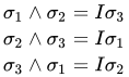
STA's even-graded elements (scalars, bivectors, pseudoscalar) form a subalgebra isomorphic to Clifford algebra Cl_3,0(R), which is equivalent to the APS or Pauli algebra. The STA bivectors are equivalent to the APS vectors and pseudovectors. The STA subalgebra becomes more explicit by renaming the STA bivectors ${\textstyle (\gamma _{1}\gamma _{0},\gamma _{2}\gamma _{0},\gamma _{3}\gamma _{0})$ as ${\textstyle (\sigma _{1},\sigma _{2},\sigma _{3})$ and the STA bivectors ${\textstyle (\gamma _{3}\gamma _{2},\gamma _{1}\gamma _{3},\gamma _{2}\gamma _{1})$ as ${\textstyle (I\sigma _{1},I\sigma _{2},I\sigma _{3})$ . The Pauli matrices, ${\textstyle {\hat {\sigma }}_{1},{\hat {\sigma }}_{2},{\hat {\sigma }}_{3}$ , are a matrix representation for ${\textstyle \sigma _{1},\sigma _{2},\sigma _{3}$ . For any pair of ${\textstyle (\sigma _{1},\sigma _{2},\sigma _{3})$ , the nonzero scalar products are ${\textstyle \sigma _{1}\cdot \sigma _{1}=\sigma _{2}\cdot \sigma _{2}=\sigma _{3}\cdot \sigma _{3}=1$ , and the nonzero exterior products are:

${\begin{aligned}\sigma _{1}\wedge \sigma _{2}&=I\sigma _{3}\\\sigma _{2}\wedge \sigma _{3}&=I\sigma _{1}\\\sigma _{3}\wedge \sigma _{1}&=I\sigma _{2}\\\end{aligned}}$

The sequence of algebra to even subalgebra continues as algebra of physical space, quaternion algebra, complex numbers and real numbers. The even STA subalgebra Cl^[0]
_(1,3)(R) of real space-time spinors in Cl_1,3(R) is isomorphic to the Clifford algebra Cl_3,0(R) of Euclidean space R³ with basis elements. See the illustration of space-time algebra spinors in Cl^[0]
_(1,3)(R) under the octonionic product as a Fano plane.

03Division

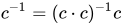
A nonzero vector ⁠ $a$ ⁠ is a null vector (degree 2 nilpotent) if ⁠ $a^{2}=0$ ⁠. An example is ⁠ $a=\gamma ^{0}+\gamma ^{1}$ ⁠. Null vectors are tangent to the light cone (null cone). An element ⁠ $b$ ⁠ is an idempotent if ⁠ $b^{2}=b$ ⁠. Two idempotents ⁠ $b_{1}$ ⁠ and ⁠ $b_{2}$ ⁠ are orthogonal idempotents if ⁠ $b_{1}b_{2}=0$ ⁠. An example of an orthogonal idempotent pair is ${\tfrac {1}{2}}(1+\gamma _{0}\gamma _{k})$ and ${\tfrac {1}{2}}(1-\gamma _{0}\gamma _{k})$ with ⁠ $k=1,2,3$ ⁠. Proper zero divisors are nonzero elements whose product is zero such as null vectors or orthogonal idempotents. A division algebra is an algebra that contains multiplicative inverse (reciprocal) elements for every element, but this occurs if there are no proper zero divisors and if the only idempotent is 1. The only associative division algebras are the real numbers, complex numbers and quaternions. As STA is not a division algebra, some STA elements may lack an inverse; however, division by the non-null vector ${\textstyle c$ may be possible by multiplication by its inverse, defined as ⁠ $c^{-1}=(c\cdot c)^{-1}c$ ⁠.

04Reciprocal frame

Associated with the orthogonal basis $\{\gamma _{0},\gamma _{1},\gamma _{2},\gamma _{3}\}$ is the reciprocal basis set $\{\gamma ^{0},\gamma ^{1},\gamma ^{2},\gamma ^{3}\}$ satisfying these equations:

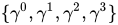
$\gamma _{\mu }\cdot \gamma ^{\nu }=\delta _{\mu }^{\nu },\quad \mu ,\nu =0,1,2,3$

These reciprocal frame vectors differ only by a sign, with ⁠ $\gamma ^{0}=\gamma _{0}$ ⁠, but ⁠ $\gamma ^{1}=-\gamma _{1}$ ⁠, ⁠ $\gamma ^{2}=-\gamma _{2}$ ⁠, ⁠ $\gamma ^{3}=-\gamma _{3}$ ⁠.

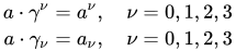
A vector ⁠ $a$ ⁠ may be represented using either the basis vectors or the reciprocal basis vectors $a=a^{\mu }\gamma _{\mu }=a_{\mu }\gamma ^{\mu }$ with summation over ⁠ $\mu =0,1,2,3$ ⁠, according to the Einstein notation. The scalar product of vector and basis vectors or reciprocal basis vectors generates the vector components.

${\begin{aligned}a\cdot \gamma ^{\nu }&=a^{\nu },\quad \nu =0,1,2,3\\a\cdot \gamma _{\nu }&=a_{\nu },\quad \nu =0,1,2,3\end{aligned}}$

The metric and index gymnastics raise or lower indices:

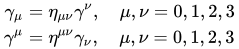
${\begin{aligned}\gamma _{\mu }&=\eta _{\mu \nu }\gamma ^{\nu },\quad \mu ,\nu =0,1,2,3\\\gamma ^{\mu }&=\eta ^{\mu \nu }\gamma _{\nu },\quad \mu ,\nu =0,1,2,3\end{aligned}}$

05Spacetime gradient

The spacetime gradient, like the gradient in a Euclidean space, is defined such that the directional derivative relationship is satisfied:

$a\cdot \nabla F(x)=\lim _{\tau \rightarrow 0}{\frac {F(x+a\tau )-F(x)}{\tau }}.$

This requires the definition of the gradient to be

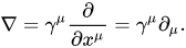
$\nabla =\gamma ^{\mu }{\frac {\partial }{\partial x^{\mu }}}=\gamma ^{\mu }\partial _{\mu }.$

Written out explicitly with ⁠ $x=ct\gamma _{0}+x^{k}\gamma _{k}$ ⁠, these partials are

$\partial _{0}={\frac {1}{c}}{\frac {\partial }{\partial t}},\quad \partial _{k}={\frac {\partial }{\partial {x^{k}}}}.$

06Space-time split

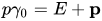
Space-time split, examples:

$x\gamma _{0}=x^{0}+\mathbf {x}$

$p\gamma _{0}=E+\mathbf {p}$

$v\gamma _{0}=\gamma (1+\mathbf {v} )$

where $\gamma$ is the Lorentz factor

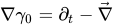
$\nabla \gamma _{0}=\partial _{t}-{\vec {\nabla }}$

In STA, a space-time split is a projection from four-dimensional space into (3+1)-dimensional space in a chosen reference frame by means of the following two operations:

a collapse of the chosen time axis, yielding a 3-dimensional space spanned by bivectors, equivalent to the standard 3-dimensional basis vectors in the algebra of physical space and
a projection of the 4D space onto the chosen time axis, yielding a 1-dimensional space of scalars, representing the scalar time.

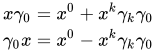
This is achieved by left-multiplication or right-multiplication by a timelike basis vector ⁠ $\gamma _{0}$ ⁠, which serves to split a four vector into a scalar timelike and a bivector spacelike component, in the reference frame co-moving with ⁠ $\gamma _{0}$ ⁠. With ⁠ $x=x^{\mu }\gamma _{\mu }$ ⁠, we have

${\begin{aligned}x\gamma _{0}&=x^{0}+x^{k}\gamma _{k}\gamma _{0}\\\gamma _{0}x&=x^{0}-x^{k}\gamma _{k}\gamma _{0}\end{aligned}}$

Space-time split is a method for representing an even-graded vector of spacetime as a vector in the Pauli algebra, an algebra where time is a scalar separated from vectors that occur in 3 dimensional space. The method replaces these spacetime vectors (⁠ $\gamma$ ⁠)

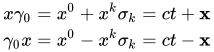
As these bivectors ⁠ $\gamma _{k}\gamma _{0}$ ⁠ square to ⁠ $1$ ⁠, they serve as a spatial basis. Utilizing the Pauli matrix notation, these are written ⁠ $\sigma _{k}=\gamma _{k}\gamma _{0}$ ⁠. Spatial vectors in STA are denoted in boldface; then with ⁠ $\mathbf {x} =x^{k}\sigma _{k}$ ⁠ and ⁠ $x^{0}=ct$ ⁠, the ⁠ $\gamma _{0}$ ⁠-space-time split ⁠ $x\gamma _{0}$ ⁠, and its reverse ⁠ $\gamma _{0}x$ ⁠ are:

${\begin{aligned}x\gamma _{0}&=x^{0}+x^{k}\sigma _{k}=ct+\mathbf {x} \\\gamma _{0}x&=x^{0}-x^{k}\sigma _{k}=ct-\mathbf {x} \end{aligned}}$

However, the above formulas only work in the Minkowski metric with signature (+ − − −). For forms of the space-time split that work in either signature, alternate definitions in which ⁠ $\sigma _{k}=\gamma _{k}\gamma ^{0}$ ⁠ and ⁠ $\sigma ^{k}=\gamma _{0}\gamma ^{k}$ ⁠ must be used.

07Transformations

To rotate a vector $v$ in geometric algebra, the following formula is used:

$v'=e^{-\beta {\frac {\theta }{2}}}\ v\ e^{\beta {\frac {\theta }{2}}}$ ,

where $\theta$ is the angle to rotate by, and ⁠ $\beta$ ⁠ is the bivector representing the plane of rotation normalized so that ⁠ $\beta {\tilde {\beta }}=1$ ⁠.

For a given spacelike bivector, ⁠ $\beta ^{2}=-1$ ⁠, so Euler's formula applies, giving the rotation

$v'=\left(\cos \left({\frac {\theta }{2}}\right)-\beta \sin \left({\frac {\theta }{2}}\right)\right)\ v\ \left(\cos \left({\frac {\theta }{2}}\right)+\beta \sin \left({\frac {\theta }{2}}\right)\right)$ .

For a given timelike bivector, ⁠ $\beta ^{2}=1$ ⁠, so a "rotation through time" uses the analogous equation for the split-complex numbers:

$v'=\left(\cosh \left({\frac {\theta }{2}}\right)-\beta \sinh \left({\frac {\theta }{2}}\right)\right)\ v\ \left(\cosh \left({\frac {\theta }{2}}\right)+\beta \sinh \left({\frac {\theta }{2}}\right)\right)$ .

Interpreting this equation, these rotations along the time direction are simply hyperbolic rotations. These are equivalent to Lorentz boosts in special relativity.

Both of these transformations are known as Lorentz transformations, and the combined set of all of them is the Lorentz group. To transform an object in STA from any basis (corresponding to a reference frame) to another, one or more of these transformations must be used.

Identifications to express Lorentz transformation formulas in terms of complex quaternions It is easy to put these Lorentz transformation formulas in terms of complex quaternions or biquaternions by making some simple identifications. The quaternion Lorentz transformations are most naturally expressed in terms of the equivalent of $X\equiv x\,\gamma _{0}=x^{0}+\gamma _{1}\,\gamma _{0}\,x^{1}+\gamma _{2}\,\gamma _{0}\,x^{2}+\gamma _{3}\,\gamma _{0}\,x^{3}=x^{0}+\sigma _{1}\,x^{1}+\sigma _{2}\,x^{2}+\sigma _{3}\,x^{3}$ Identify the pseudoscalar $\gamma _{0}\gamma _{1}\gamma _{2}\gamma _{3}$ as ⁠ $i$ ⁠, the square root of ⁠ $-1$ ⁠. The square of the pseudoscalar $\gamma _{0}\gamma _{1}\gamma _{2}\gamma _{3}\,$ is -1 and it commutes with scalars and bivectors, which is what $X$ is and what the transformation operators are.

Define ${\textbf {I}},\,{\textbf {J}},\,{\textbf {K}}$ to be the basis quaternions such that ${\textbf {I}}\,{\textbf {I}}={\textbf {J}}\,{\textbf {J}}={\textbf {K}}\,{\textbf {K}}={\textbf {I}}\,{\textbf {J}}\,{\textbf {K}}=-1\;$ In this discussion ${\textbf {I}}$ is a basis quaternion. Identify $-i\sigma _{1}\rightarrow {\textbf {I}}\quad -i\sigma _{2}\rightarrow {\textbf {J}}\quad -i\sigma _{3}\rightarrow {\textbf {K}}\quad$ .

For the bivector ⁠ $\beta$ ⁠ having a time axis, such as $\gamma _{1}\gamma _{0},$ $e^{\beta \,{\frac {\alpha }{2}}}\,\gamma _{0}=\gamma _{0}\,e^{-\beta \,{\frac {\alpha }{2}}}$ . Here, ⁠ $\alpha$ ⁠ is a real scalar parameter.

For the bivector ⁠ $\beta$ ⁠ having two space axes, such as $\gamma _{2}\,\gamma _{3},$ $e^{\beta \,{\frac {\theta }{2}}}\,\gamma _{0}=\gamma _{0}\,e^{\beta \,{\frac {\theta }{2}}}$ . Here, ⁠ $\theta$ ⁠ is a real scalar parameter.

For a spatial rotation about the x-axis $\beta =\gamma _{2}\,\gamma _{3}=-(\gamma _{0}\,\gamma _{1}\,\gamma _{2}\,\gamma _{3})\,\gamma _{1}\,\gamma _{0}\rightarrow -i\,\sigma _{1}\rightarrow {\textbf {I}}$ , giving ${\textbf {X}}'\,=\,e^{-{\frac {\theta }{2}}\,{\textbf {I}}}\,{\textbf {X}}\,e^{{\frac {\theta }{2}}\,{\textbf {I}}}\quad$ Here, ⁠ $\theta$ ⁠ is the angle of rotation and ${\textbf {X}}=x^{0}+i\,x^{1}{\textbf {I}}+i\,x^{2}{\textbf {J}}+i\,x^{3}{\textbf {K}}$ . This is the form used by P. A. M. Dirac.

For a boost in the x-direction, the bivector $\beta =\gamma _{1}\,\gamma _{0}\rightarrow \sigma _{1}\rightarrow i\,{\textbf {I}}$ , giving ${\textbf {X}}'\,=\,e^{-{\frac {\alpha }{2}}\,i\,{\textbf {I}}}\,{\textbf {X}}\,e^{-{\frac {\alpha }{2}}\,i\,{\textbf {I}}}\quad$ Here ⁠ $\cosh \alpha =(1-v^{2}/c^{2})^{-1/2}$ ⁠, where ⁠ $v$ ⁠ is the velocity.

Any spacetime element ⁠ $A$ ⁠ is transformed by multiplication with the pseudoscalar to form its Hodge dual ⁠ $AI$ ⁠. Duality rotation transforms spacetime element ⁠ $A$ ⁠ to element ⁠ $A^{\prime }$ ⁠ through angle ⁠ $\phi$ ⁠ with pseudoscalar ⁠ $I$ ⁠ is:

$A^{\prime }=e^{I\phi }A.$

Duality rotation occurs only for non-singular Clifford algebra, non-singular meaning a Clifford algebra containing pseudoscalars with a non-zero square.

Grade involution (main involution, inversion) transforms every ⁠ $r$ ⁠-vector ⁠ $A_{r}$ ⁠ to ⁠ $A_{r}^{\ast }$ ⁠:

$A_{r}^{\ast }=(-1)^{r}\ A_{r}.$

Reversion transformation occurs by decomposing any spacetime element as a sum of products of vectors and then reversing the order of each product. For multivector ${\textstyle A$ arising from a product of vectors, ${\textstyle a_{1}a_{2}\ldots a_{r-1}a_{r}$ the reversion is ${\textstyle A^{\dagger }$ :

$A=a_{1}a_{2}\ldots a_{r-1}a_{r},\quad A^{\dagger }=a_{r}a_{r-1}\ldots a_{2}a_{1}.$

Clifford conjugation of a spacetime element ⁠ $A$ ⁠ combines reversion and grade involution transformations, indicated as ⁠ ${\tilde {A}}$ ⁠:

${\tilde {A}}=A^{\ast \dagger }$

The grade involution, reversion and Clifford conjugation transformations are involutions.

08Classical electromagnetism

Faraday bivector

In STA, the electric field and magnetic field can be unified into a single bivector field, known as the Faraday bivector, equivalent to the Faraday tensor. It is defined as:

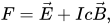
$F={\vec {E}}+Ic{\vec {B}},$

where $E$ and $B$ are the usual electric and magnetic fields, and $I$ is the STA pseudoscalar. Alternatively, expanding $F$ in terms of components, $F$ is defined that

$F=E^{i}\sigma _{i}+IcB^{i}\sigma _{i}=E^{1}\gamma _{1}\gamma _{0}+E^{2}\gamma _{2}\gamma _{0}+E^{3}\gamma _{3}\gamma _{0}-cB^{1}\gamma _{2}\gamma _{3}-cB^{2}\gamma _{3}\gamma _{1}-cB^{3}\gamma _{1}\gamma _{2}.$

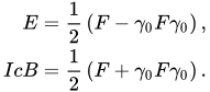
The separate ${\vec {E}}$ and ${\vec {B}}$ fields are recovered from $F$ using

${\begin{aligned}E={\frac {1}{2}}\left(F-\gamma _{0}F\gamma _{0}\right),\\IcB={\frac {1}{2}}\left(F+\gamma _{0}F\gamma _{0}\right).\end{aligned}}$

The ⁠ $\gamma _{0}$ ⁠ term represents a given reference frame, and as such, using different reference frames will result in apparently different relative fields, exactly as in standard special relativity.

Since the Faraday bivector is a relativistic invariant, further information can be found in its square, giving two new Lorentz-invariant quantities, one scalar, and one pseudoscalar:

$F^{2}=E^{2}-c^{2}B^{2}+2Ic{\vec {E}}\cdot {\vec {B}}.$

The scalar part corresponds to the Lagrangian density for the electromagnetic field, and the pseudoscalar part is a less-often seen Lorentz invariant.

Maxwell's equation

STA formulates Maxwell's equations in a simpler form as one equation, rather than the 4 equations of vector calculus. Similarly to the above field bivector, the electric charge density and current density can be unified into a single spacetime vector, equivalent to a four-vector. As such, the spacetime current ⁠ $J$ ⁠ is given by

$J=c\rho \gamma _{0}+J^{i}\gamma _{i},$

where the components ⁠ $J^{i}$ ⁠ are the components of the classical 3-dimensional current density. When combining these quantities in this way, it makes it particularly clear that the classical charge density is nothing more than a current travelling in the timelike direction given by ⁠ $\gamma _{0}$ ⁠.

Combining the electromagnetic field and current density together with the spacetime gradient as defined earlier, we can combine all four of Maxwell's equations into a single equation in STA.

Maxwell's equation:

$\nabla F=\mu _{0}cJ$

The fact that these quantities are all covariant objects in the STA automatically ensures Lorentz covariance of the equation, which is much easier to show than when separated into four separate equations.

In this form, it is also much simpler to prove certain properties of Maxwell's equations, such as the conservation of charge. Using the fact that for any bivector field, the divergence of its spacetime gradient is ⁠ $0$ ⁠, one can perform the following manipulation:

${\begin{aligned}\nabla \cdot \left[\nabla F\right]&=\nabla \cdot \left[\mu _{0}cJ\right]\\0&=\nabla \cdot J.\end{aligned}}$

This equation has the clear meaning that the divergence of the current density is zero, i.e. the total charge and current density over time is conserved.

Using the electromagnetic field, the form of the Lorentz force on a charged particle can also be considerably simplified using STA.

Lorentz force on a charged particle:

${\mathcal {F}}=qF\cdot v$

Potential formulation

In the standard vector calculus formulation, two potential functions are used: the electric scalar potential, and the magnetic vector potential. Using the tools of STA, these two objects are combined into a single vector field $A$ , analogous to the electromagnetic four-potential in tensor calculus. In STA, it is defined as

$A={\frac {\phi }{c}}\gamma _{0}+A^{k}\gamma _{k},$

where ⁠ $\phi$ ⁠ is the scalar potential, and ⁠ $A^{k}$ ⁠ are the components of the magnetic potential.

The electromagnetic field can also be expressed in terms of this potential field, using

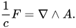
${\frac {1}{c}}F=\nabla \wedge A.$

However, this definition is not unique. For any twice-differentiable scalar function ⁠ $\Lambda ({\vec {x}})$ ⁠, the potential given by

$A'=A+\nabla \Lambda$

will also give the same $F$ as the original, due to the fact that

$\nabla \wedge \left(A+\nabla \Lambda \right)=\nabla \wedge A+\nabla \wedge \nabla \Lambda =\nabla \wedge A.$

This phenomenon is called gauge freedom. The process of choosing a suitable function ⁠ $\Lambda$ ⁠ to make a given problem simplest is known as gauge fixing. However, in relativistic electrodynamics, the Lorenz condition is often imposed, where ⁠ $\nabla \cdot {\vec {A}}=0$ ⁠.

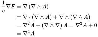
To reformulate the STA Maxwell equation in terms of the potential ⁠ $A$ ⁠, ⁠ $F$ ⁠ is first replaced with the above definition.

${\begin{aligned}{\frac {1}{c}}\nabla F&=\nabla \left(\nabla \wedge A\right)\\&=\nabla \cdot \left(\nabla \wedge A\right)+\nabla \wedge \left(\nabla \wedge A\right)\\&=\nabla ^{2}A+\left(\nabla \wedge \nabla \right)A=\nabla ^{2}A+0\\&=\nabla ^{2}A\end{aligned}}$

Substituting in this result, one arrives at the potential formulation of electromagnetism in STA:

Potential equation:

$\nabla ^{2}A=\mu _{0}J$

Lagrangian formulation

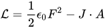
Analogously to the tensor calculus formalism, the potential formulation in STA naturally leads to an appropriate Lagrangian density.

Electromagnetic Lagrangian density:

${\mathcal {L}}={\frac {1}{2}}\epsilon _{0}F^{2}-J\cdot A$

The multivector-valued Euler-Lagrange equations for the field can be derived, and being loose with the mathematical rigor of taking the partial derivative with respect to something that is not a scalar, the relevant equations become:

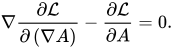
$\nabla {\frac {\partial {\mathcal {L}}}{\partial \left(\nabla A\right)}}-{\frac {\partial {\mathcal {L}}}{\partial A}}=0.$

To begin to re-derive the potential equation from this form, it is simplest to work in the Lorenz gauge, setting

$\nabla \cdot A=0.$

This process can be done regardless of the chosen gauge, but this makes the resulting process considerably clearer. Due to the structure of the geometric product, using this condition results in ⁠ $\nabla \wedge A=\nabla A$ ⁠.

After substituting in ⁠ $F=c\nabla A$ ⁠, the same equation of motion as above for the potential field ⁠ $A$ ⁠ is easily obtained.

09Pauli equation

STA allows the description of the Pauli particle in terms of a real theory in place of a matrix theory. The matrix theory description of the Pauli particle is:

$i\hbar \,\partial _{t}\Psi =H_{S}\Psi -{\frac {e\hbar }{2mc}}\,{\hat {\sigma }}\cdot \mathbf {B} \Psi ,$

where ⁠ $\Psi$ ⁠ is a spinor, ⁠ $i$ ⁠ is the imaginary unit with no geometric interpretation, ⁠ ${\hat {\sigma }}_{i}$ ⁠ are the Pauli matrices (with the 'hat' notation indicating that ⁠ ${\hat {\sigma }}$ ⁠ is a matrix operator and not an element in the geometric algebra), and ⁠ $H_{S}$ ⁠ is the Schrödinger Hamiltonian.

The STA approach transforms the matrix spinor representation ⁠ $\vert \psi \rangle$ ⁠ to the STA representation ⁠ $\psi$ ⁠ using elements, ${\textstyle \sigma _{1},\sigma _{2},\sigma _{3}$ , of the even-graded spacetime subalgebra and the pseudoscalar ⁠ $I=\sigma _{1}\sigma _{2}\sigma _{3}$ ⁠:

$|\psi \rangle ={\begin{bmatrix}\operatorname {cos(\theta /2)\ e^{-i\phi /2}} \\\operatorname {sin(\theta /2)\ e^{+i\phi /2}} \end{bmatrix}}={\begin{bmatrix}a^{0}+ia^{3}\\-a^{2}+ia^{1}\end{bmatrix}}\mapsto \psi =a^{0}+a^{1}\mathbf {I\sigma _{1}} +a^{2}\mathbf {I\sigma _{2}} +a^{3}\mathbf {I\sigma _{3}}$

The Pauli particle is described by the real Pauli-Schrödinger equation:

$\partial _{t}\psi \,I\sigma _{3}\,\hbar =H_{S}\psi -{\frac {e\hbar }{2mc}}\,\mathbf {B} \psi \sigma _{3},$

where now ⁠ $\psi$ ⁠ is an even multi-vector of the geometric algebra, and the Schrödinger Hamiltonian is ⁠ $H_{S}$ ⁠. Hestenes refers to this as the real Pauli-Schrödinger theory to emphasize that this theory reduces to the Schrödinger theory if the term that includes the magnetic field is dropped. The vector ⁠ $\sigma _{3}$ ⁠ is an arbitrarily selected fixed vector; a fixed rotation can generate any alternative selected fixed vector ⁠ $\sigma _{3}^{\prime }$ ⁠.

10Dirac equation

STA enables a description of the Dirac particle in terms of a real theory in place of a matrix theory. The matrix theory description of the Dirac particle is:

${\hat {\gamma }}^{\mu }(i\partial _{\mu }-e\mathbf {A} _{\mu })|\psi \rangle =m|\psi \rangle ,$

where ⁠ ${\hat {\gamma }}$ ⁠ are the Dirac matrices and ⁠ $i$ ⁠ is the imaginary unit with no geometric interpretation.

Using the same approach as for Pauli equation, the STA approach transforms the matrix upper spinor ⁠ $\vert \psi _{U}\rangle$ ⁠ and matrix lower spinor ⁠ $\vert \psi _{L}\rangle$ ⁠ of the matrix Dirac spinor⁠ $\vert \psi \rangle$ ⁠ to the corresponding geometric algebra spinor representations ⁠ $\psi _{U}$ ⁠ and ⁠ $\psi _{L}$ ⁠. These are then combined to represent the full geometric algebra Dirac spinor ⁠ $\psi$ ⁠.

$|\psi \rangle ={\begin{vmatrix}|\psi _{U}\rangle \\|\psi _{L}\rangle \end{vmatrix}}\mapsto \psi =\psi _{U}+\psi _{L}\mathbf {\sigma _{3}}$

Following Hestenes' derivation, the Dirac particle is described by the equation:

Dirac equation in STA:

$\nabla \psi \,I\sigma _{3}-e\mathbf {A} \psi =m\psi \gamma _{0}$

Here, ⁠ $\psi$ ⁠ is the spinor field, ⁠ $\gamma _{0}$ ⁠ and ⁠ $I\sigma _{3}$ ⁠ are elements of the geometric algebra, ⁠ $\mathbf {A}$ ⁠ is the electromagnetic four-potential, and ⁠ $\nabla =\gamma ^{\mu }\partial _{\mu }$ ⁠ is the spacetime vector derivative.

Dirac spinors

A relativistic Dirac spinor ${\textstyle \psi$ can be expressed as:

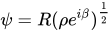
$\psi =R(\rho e^{i\beta })^{\frac {1}{2}}$

where, according to its derivation by David Hestenes, ⁠ $\psi =\psi (x)$ ⁠ is an even multivector-valued function on spacetime, ⁠ $R=R(x)$ ⁠ is a unimodular spinor or "rotor", and ⁠ $\rho =\rho (x)$ ⁠ and ⁠ $\beta =\beta (x)$ ⁠ are scalar-valued functions. In this construction, the components of ⁠ $\psi$ ⁠ directly correspond with the components of a Dirac spinor, both having 8 scalar degrees of freedom.

This equation is interpreted as connecting spin with the imaginary pseudoscalar.

The rotor, ⁠ $R$ ⁠, Lorentz transforms the frame of vectors ⁠ $\gamma _{\mu }$ ⁠ into another frame of vectors ⁠ $e_{\mu }$ ⁠ by the operation ⁠ $e_{\mu }=R\gamma _{\mu }R^{\dagger }$ ⁠; note that ⁠ $R^{\dagger }$ ⁠ indicates the reverse transformation.

This has been extended to provide a framework for locally varying vector- and scalar-valued observables and support for the zitterbewegung interpretation of quantum mechanics originally proposed by Schrödinger.

Hestenes has compared his expression for ⁠ $\psi$ ⁠ with Feynman's expression for it in the path integral formulation:

$\psi =e^{i\Phi _{\lambda }/\hbar },$

where ⁠ $\Phi _{\lambda }$ ⁠ is the classical action along the ⁠ $\lambda$ ⁠-path.

Using the spinors, the current density from the field can be expressed by

$J^{\mu }={\bar {\psi }}\gamma ^{\mu }\psi$

Symmetries

Global phase symmetry is a constant global phase shift of the wave function that leaves the Dirac equation unchanged. Local phase symmetry is a spatially varying phase shift that leaves the Dirac equation unchanged if accompanied by a gauge transformation of the electromagnetic four-potential as expressed by these combined substitutions.

$\psi \mapsto \psi e^{\alpha (x)I\sigma _{3}},\quad eA\mapsto eA-\nabla \alpha (x)$

In these equations, the local phase transformation is a phase shift ⁠ $\alpha (x)$ ⁠ at spacetime location ⁠ $x$ ⁠ with pseudovector ⁠ $I$ ⁠ and ⁠ $\sigma _{3}$ ⁠ of even-graded spacetime subalgebra applied to wave function ⁠ $\psi$ ⁠; the gauge transformation is a subtraction of the gradient of the phase shift ⁠ $\nabla \alpha (x)$ ⁠ from the electromagnetic four-potential ⁠ $A$ ⁠ with particle electric charge ⁠ $e$ ⁠.

Researchers have applied STA and related Clifford algebra approaches to gauge theories, electroweak interaction, Yang-Mills theory, and the Standard Model.

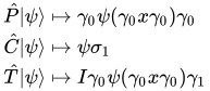
The discrete symmetries are parity (⁠ ${\hat {P}}$ ⁠), charge conjugation (⁠ ${\hat {C}}$ ⁠) and time reversal (⁠ ${\hat {T}}$ ⁠) applied to wave function ⁠ $\psi$ ⁠. These effects are:

${\begin{aligned}{\hat {P}}|\psi \rangle &\mapsto \gamma _{0}\psi (\gamma _{0}x\gamma _{0})\gamma _{0}\\{\hat {C}}|\psi \rangle &\mapsto \psi \sigma _{1}\\{\hat {T}}|\psi \rangle &\mapsto I\gamma _{0}\psi (\gamma _{0}x\gamma _{0})\gamma _{1}\end{aligned}}$

11General relativity

General relativity

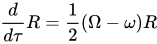
Researchers have applied STA and related Clifford algebra approaches to relativity, gravity and cosmology. The gauge theory gravity (GTG) uses STA to describe an induced curvature on Minkowski space while admitting a gauge symmetry under "arbitrary smooth remapping of events onto spacetime" leading to this geodesic equation.

${\frac {d}{d\tau }}R={\frac {1}{2}}(\Omega -\omega )R$

and the covariant derivative

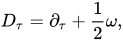
$D_{\tau }=\partial _{\tau }+{\frac {1}{2}}\omega ,$

where ⁠ $\omega$ ⁠ is the connection associated with the gravitational potential, and ⁠ $\Omega$ ⁠ is an external interaction such as an electromagnetic field.

The theory shows some promise for the treatment of black holes, as its form of the Schwarzschild solution does not break down at singularities; most of the results of general relativity have been mathematically reproduced, and the relativistic formulation of classical electrodynamics has been extended to quantum mechanics and the Dirac equation.

Watch videos about Spacetime algebraExplainers and documentaries on YouTube (opens in a new tab)

Sources and credits

This article is adapted from the Wikipedia article “Spacetime algebra”, written by its contributors and licensed under CC BY-SA 4.0. Fathomly has changed the layout, removed citation markers, navigation and maintenance notices, and adjusted punctuation. This adapted version is shared under the same license. For references, see the original article.

Images, from Wikimedia Commons:

Space-Time-Algebra-FanoPlane.svg by Jgmoxness, CC BY 4.0
Spacetime Algebra Octonion Multiplication Tables.svg by Jgmoxness, CC BY-SA 4.0

Fathomly is not affiliated with or endorsed by the Wikimedia Foundation. Spotted a problem? Tell us.