Encyclopedia

Electric potential

Line integral of the electric field

Wikipedia contributorsAdapted for Fathomly · View authors

8 min read
Source updated July 29, 2026

Electric potential, also known as the electrostatic potential or electric field potential, is a field of scalar quantities through space, often denoted with the letter $\varphi$ or $V$ , that gives, for each point in space, the electric potential energy per unit of electric charge that a point charge would have if it was located at that point: at every point, a particle of charge $q_{\text{particle}}$ would have the electric potential energy $U_{\text{particle when at the point}}=q_{\text{particle}}\,V_{\text{point}}$ . The difference in electric potential energy U, $U=U_{B}-U_{A}$ , that a charged particle of charge $q$ would have between two points $A$ and $B$ in a static electric field, equals $q$ times the difference $V_{B}-V_{A}$ of the electric potentials at A and B: $U_{B}-U_{A}=q\times (V_{B}-V_{A})$ . More precisely, electric potential is the amount of work needed to move a test charge from a reference point to a specific point in a static electric field, normalized to a unit of charge. The test charge used is small enough that disturbance to the field-producing charges is unnoticeable, and its motion across the field is supposed to proceed with negligible acceleration, so as to avoid the test charge acquiring kinetic energy or producing radiation. By definition, the electric potential at the reference point is zero units. Typically, the reference point is earth or a point at infinity, although any point can be used.

In classical electrostatics, the electrostatic field is a vector quantity expressed as the gradient of the electrostatic potential, which is a scalar quantity denoted by V or occasionally φ, equal to the electric potential energy of any charged particle at any location (measured in joules) divided by the charge of that particle (measured in coulombs). By dividing out the charge on the particle a quotient is obtained that is a property of the electric field itself. In short, an electric potential is the electric potential energy per unit charge.

This value can be calculated in either a static (time-invariant) or a dynamic (time-varying) electric field at a specific time with the unit joules per coulomb (J⋅C⁻¹) or volt (V). The electric potential at infinity is assumed to be zero.

In electrodynamics, when time-varying fields are present, the electric field cannot be expressed only as a scalar potential. Instead, the electric field can be expressed as both the scalar electric potential and the magnetic vector potential. The electric potential and the magnetic vector potential together form a four-vector, so that the two kinds of potential are mixed under Lorentz transformations.

Practically, the electric potential is a continuous function in all space, because a spatial derivative of a discontinuous electric potential yields an electric field of impossibly infinite magnitude. Notably, the electric potential due to an idealized point charge (proportional to 1 ⁄ r, with r the distance from the point charge) is continuous in all space except at the location of the point charge. Though electric field is not continuous across an idealized surface charge, it is not infinite at any point. Therefore, the electric potential is continuous across an idealized surface charge. Additionally, an idealized line of charge has electric potential (proportional to ln(r), with r the radial distance from the line of charge) is continuous everywhere except on the line of charge.

01Introduction

Classical mechanics explores concepts such as force, energy, and potential. Force and potential energy are directly related. A net force acting on any object will cause it to accelerate. As an object moves in the direction of a force acting on it, its potential energy decreases. For example, the gravitational potential energy of a cannonball at the top of a hill is greater than at the base of the hill. As it rolls downhill, its potential energy decreases and is being translated to motion, kinetic energy.

It is possible to define the potential of certain force fields so that the potential energy of an object in that field depends only on the position of the object with respect to the field. Two such force fields are a gravitational field and an electric field (in the absence of time-varying magnetic fields). Such fields affect objects because of the intrinsic properties (e.g., mass or charge) and positions of the objects.

An object may possess a property known as electric charge. Since an electric field exerts force on a charged object, if the object has a positive charge, the force will be in the direction of the electric field vector at the location of the charge; if the charge is negative, the force will be in the opposite direction.

The magnitude of force is given by the quantity of the charge multiplied by the magnitude of the electric field vector,

$|\mathbf {F} |=q|\mathbf {E} |.$

02Electrostatics

An electric potential at a point r in a static electric field E is given by the line integral

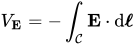
$V_{\mathbf {E} }=-\int _{\mathcal {C}}\mathbf {E} \cdot \mathrm {d} {\boldsymbol {\ell }}\,$

where C is an arbitrary path from some fixed reference point to r; it is uniquely determined up to a constant that is added or subtracted from the integral. In electrostatics, the Maxwell-Faraday equation reveals that the curl ${\textstyle \nabla \times \mathbf {E}$ is zero, making the electric field conservative. Thus, the line integral above does not depend on the specific path C chosen but only on its endpoints, making ${\textstyle V_{\mathbf {E} }$ well-defined everywhere. The gradient theorem then allows us to write:

$\mathbf {E} =-\mathbf {\nabla } V_{\mathbf {E} }\,$

This states that the electric field points "downhill" towards lower voltages. By Gauss's law, the potential can also be found to satisfy Poisson's equation: $\mathbf {\nabla } \cdot \mathbf {E} =\mathbf {\nabla } \cdot \left(-\mathbf {\nabla } V_{\mathbf {E} }\right)=-\nabla ^{2}V_{\mathbf {E} }=\rho /\varepsilon _{0}$

where ρ is the total charge density and ${\textstyle \mathbf {\nabla } \cdot$ denotes the divergence.

The concept of electric potential is closely linked with potential energy. A test charge, q, has an electric potential energy, U_E, given by

$U_{\mathbf {E} }=q\,V.$

The potential energy and hence, also the electric potential, is only defined up to an additive constant: one must arbitrarily choose a position where the potential energy and the electric potential are zero.

These equations cannot be used if ${\textstyle \nabla \times \mathbf {E} \neq \mathbf {0}$ , i.e., in the case of a non-conservative electric field (caused by a changing magnetic field; see Maxwell's equations). The generalization of electric potential to this case is described in the section § Generalization to electrodynamics.

Electric potential due to a point charge

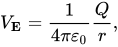
The electric potential arising from a point charge, Q, at a distance, r, from the location of Q is observed to be $V_{\mathbf {E} }={\frac {1}{4\pi \varepsilon _{0}}}{\frac {Q}{r}},$ where ε₀ is the permittivity of vacuum, V_E is known as the Coulomb potential. Note that, in contrast to the magnitude of an electric field due to a point charge, the electric potential scales respective to the reciprocal of the radius, rather than the radius squared.

The electric potential at any location, r, in a system of point charges is equal to the sum of the individual electric potentials due to every point charge in the system. This fact simplifies calculations significantly, because addition of potential (scalar) fields is much easier than addition of the electric (vector) fields. Specifically, the potential of a set of discrete point charges q_i at points r_i becomes

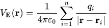
$V_{\mathbf {E} }(\mathbf {r} )={\frac {1}{4\pi \varepsilon _{0}}}\sum _{i=1}^{n}{\frac {q_{i}}{|\mathbf {r} -\mathbf {r} _{i}|}}\,$

where

r is a point at which the potential is evaluated;
r_i is a point at which there is a nonzero charge; and
q_i is the charge at the point r_i.

And the potential of a continuous charge distribution ρ(r) becomes

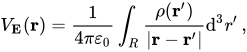
$V_{\mathbf {E} }(\mathbf {r} )={\frac {1}{4\pi \varepsilon _{0}}}\int _{R}{\frac {\rho (\mathbf {r} ')}{|\mathbf {r} -\mathbf {r} '|}}\mathrm {d} ^{3}r'\,,$

where

r is a point at which the potential is evaluated;
R is a region containing all the points at which the charge density is nonzero;
r' is a point inside R; and
ρ(r') is the charge density at the point r'.

The equations given above for the electric potential (and all the equations used here) are in the forms required by SI units. In some other (less common) systems of units, such as CGS-Gaussian, many of these equations would be altered.

03Generalization to electrodynamics

When time-varying magnetic fields are present (which is true whenever there are time-varying electric fields and vice versa), it is not possible to describe the electric field simply as a scalar potential V because the electric field is no longer conservative: $\textstyle \int _{C}\mathbf {E} \cdot \mathrm {d} {\boldsymbol {\ell }}$ is path-dependent because $\mathbf {\nabla } \times \mathbf {E} \neq \mathbf {0}$ (due to the Maxwell-Faraday equation).

Instead, one can still define a scalar potential by also including the magnetic vector potential A. In particular, A is defined to satisfy:

$\mathbf {B} =\mathbf {\nabla } \times \mathbf {A}$

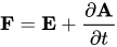
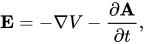
where B is the magnetic field. By the fundamental theorem of vector calculus, such an A can always be found, since the divergence of the magnetic field is always zero due to the absence of magnetic monopoles. Now, the quantity $\mathbf {F} =\mathbf {E} +{\frac {\partial \mathbf {A} }{\partial t}}$ is a conservative field, since the curl of $\mathbf {E}$ is canceled by the curl of ${\frac {\partial \mathbf {A} }{\partial t}}$ according to the Maxwell-Faraday equation. One can therefore write $\mathbf {E} =-\mathbf {\nabla } V-{\frac {\partial \mathbf {A} }{\partial t}},$

where V is the scalar potential defined by the conservative field F.

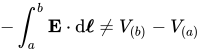
The electrostatic potential is simply the special case of this definition where A is time-invariant. On the other hand, for time-varying fields, $-\int _{a}^{b}\mathbf {E} \cdot \mathrm {d} {\boldsymbol {\ell }}\neq V_{(b)}-V_{(a)}$ unlike electrostatics.

Gauge freedom

The electrostatic potential could have any constant added to it without affecting the electric field. In electrodynamics, the electric potential has infinitely many degrees of freedom. For any (possibly time-varying or space-varying) scalar field, 𝜓, we can perform the following gauge transformation to find a new set of potentials that produce exactly the same electric and magnetic fields:

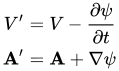
${\begin{aligned}V^{\prime }&=V-{\frac {\partial \psi }{\partial t}}\\\mathbf {A} ^{\prime }&=\mathbf {A} +\nabla \psi \end{aligned}}$

Given different choices of gauge, the electric potential could have quite different properties. In the Coulomb gauge, the electric potential is given by Poisson's equation

$\nabla ^{2}V=-{\frac {\rho }{\varepsilon _{0}}}$

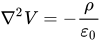
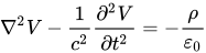
just like in electrostatics. However, in the Lorenz gauge, the electric potential is a retarded potential that propagates at the speed of light and is the solution to an inhomogeneous wave equation:

$\nabla ^{2}V-{\frac {1}{c^{2}}}{\frac {\partial ^{2}V}{\partial t^{2}}}=-{\frac {\rho }{\varepsilon _{0}}}$

04Units

The SI derived unit of electric potential is the volt (in honor of Alessandro Volta), denoted as V, which is why the electric potential difference between two points in space is known as a voltage. Older units are rarely used today. Variants of the centimetre-gram-second system of units included a number of different units for electric potential, including the abvolt and the statvolt.

05Galvani potential versus electrochemical potential

Inside metals (and other solids and liquids), the energy of an electron is affected not only by the electric potential, but also by the specific atomic environment that it is in. When a voltmeter is connected between two different types of metal, it measures the potential difference corrected for the different atomic environments. The quantity measured by a voltmeter is called electrochemical potential or fermi level, while the pure unadjusted electric potential, V, is sometimes called the Galvani potential, ϕ. The terms "voltage" and "electric potential" are a bit ambiguous but one may refer to either of these in different contexts.

06Common formulas


Charge configuration	Electric potential
Infinite wire	$V=-{\frac {\lambda }{2\pi \varepsilon _{0}}}\ln x,$ where $\lambda$ is uniform linear charge density.
Infinitely large surface	$V=-{\frac {\sigma x}{2\varepsilon _{0}}},$ where $\sigma$ is uniform surface charge density.
Infinitely long cylindrical volume	$V=-{\frac {\lambda }{2\pi \varepsilon _{0}}}\ln x,$ where $\lambda$ is uniform linear charge density.
Spherical volume	$V={\frac {Q}{4\pi \varepsilon _{0}x}},$ outside the sphere, where $Q$ is the total charge uniformly distributed in the volume.	$V={\frac {Q(3R^{2}-r^{2})}{8\pi \varepsilon _{0}R^{3}}},$ inside the sphere, where $Q$ is the total charge uniformly distributed in the volume.
Spherical surface	$V={\frac {Q}{4\pi \varepsilon _{0}x}},$ outside the sphere, where $Q$ is the total charge uniformly distributed on the surface.	$V={\frac {Q}{4\pi \varepsilon _{0}R}},$ inside the sphere for uniform charge distribution.
Charged Ring	$V={\frac {Q}{4\pi \varepsilon _{0}{\sqrt {R^{2}+x^{2}}}}},$ on the axis, where $Q$ is the total charge uniformly distributed on the ring.
Charged Disc	$V={\frac {\sigma }{2\varepsilon _{0}}}\left[{\sqrt {x^{2}+R^{2}}}-x\right],$ on the axis, where $\sigma$ is the uniform surface charge density.
Electric Dipole	$V=0,$ on the equatorial plane.	$V={\frac {p}{4\pi \varepsilon _{0}x^{2}}},$ on the axis (given that $x\gg d$ ), where $x$ can also be negative to indicate position at the opposite direction on the axis, and $p$ is the magnitude of electric dipole moment.

Watch videos about Electric potentialExplainers and documentaries on YouTube (opens in a new tab)

Sources and credits

This article is adapted from the Wikipedia article “Electric potential”, written by its contributors and licensed under CC BY-SA 4.0. Fathomly has changed the layout, removed citation markers, navigation and maintenance notices, and adjusted punctuation. This adapted version is shared under the same license. For references, see the original article.

Images, from Wikimedia Commons:

VFPt metal balls largesmall potential+contour.svg by Geek3, CC BY-SA 4.0
Electric potential varying charge.gif by Lookang, CC BY-SA 3.0

Fathomly is not affiliated with or endorsed by the Wikimedia Foundation. Spotted a problem? Tell us.