Encyclopedia

Rectangular function

Function whose graph is 0, then 1, then 0 again, in an almost-everywhere continuous way

Wikipedia contributorsAdapted for Fathomly · View authors

2 min read
Source updated June 5, 2026

The rectangular function (also known as the rectangle function, rect function, Pi function, Heaviside Pi function, gate function, unit pulse, or the normalized boxcar function) is defined as

$\operatorname {rect} \left({\frac {t}{T}}\right)=\Pi \left({\frac {t}{T}}\right)=\left\{{\begin{array}{rl}0,&{\text{if }}|t|>{\frac {T}{2}}\\{\frac {1}{2}},&{\text{if }}|t|={\frac {T}{2}}\\1,&{\text{if }}|t|<{\frac {T}{2}}.\end{array}}\right.$

Alternative definitions of the function define ${\textstyle \operatorname {rect} \left(t=\pm {\frac {T}{2}}\right)$ to be 0, 1, or undefined. The area under the curve does not change for the different definitions of the functions at ${\textstyle t=\pm {\frac {T}{2}}$ .

The rectangular function can be used as the basis for a rectangular wave.

01History

The rect function has been introduced 1953 by Woodward in "Probability and Information Theory, with Applications to Radar" as an ideal cutout operator, together with the sinc function as an ideal interpolation operator, and their counter operations which are sampling (comb operator) and replicating (rep operator), respectively.

02Relation to the boxcar function

The rectangular function is a special case of the more general boxcar function:

$\operatorname {rect} \left({\frac {t-X}{Y}}\right)=H(t-(X-Y/2))-H(t-(X+Y/2))=H(t-X+Y/2)-H(t-X-Y/2)$

where $H(x)$ is the Heaviside step function; the function is centered at $X$ and has duration $Y$ , from $X-Y/2$ to $X+Y/2.$

03Fourier transform of the rectangular function

The unitary Fourier transforms of the rectangular function are $\int _{-\infty }^{\infty }\operatorname {rect} (t)\cdot e^{-i2\pi ft}\,dt={\frac {\sin(\pi f)}{\pi f}}=\operatorname {sinc} (\pi f)=\operatorname {sinc} _{\pi }(f),$ using ordinary frequency f, where $\operatorname {sinc} _{\pi }$ is the normalized form of the sinc function and ${\frac {1}{\sqrt {2\pi }}}\int _{-\infty }^{\infty }\operatorname {rect} (t)\cdot e^{-i\omega t}\,dt={\frac {1}{\sqrt {2\pi }}}\cdot {\frac {\sin \left(\omega /2\right)}{\omega /2}}={\frac {1}{\sqrt {2\pi }}}\cdot \operatorname {sinc} \left(\omega /2\right),$ using angular frequency $\omega$ , where $\operatorname {sinc}$ is the unnormalized form of the sinc function.

For $\operatorname {rect} (x/a)$ , its Fourier transform is $\int _{-\infty }^{\infty }\operatorname {rect} \left({\frac {t}{a}}\right)\cdot e^{-i2\pi ft}\,dt=a{\frac {\sin(\pi af)}{\pi af}}=a\ \operatorname {sinc} _{\pi }{(af)}.$

04Self convolution of the Rectangular function

The self convolution of the dis-continuous rectangular function results in the triangular function, a piecewise defined spline that is continuous, but not continuously differentiable. Successive convolutions of the rectangular function result in piecewise defined pulses with lower maximums which are wider and smoother, with "smoother" meaning higher-order derivatives are continuous.

A convolution of the discontinuous rectangular function with itself results in the triangular function, which is a continuous function:

${\begin{aligned}\operatorname {rect(2t/T)} *\operatorname {rect(2t/T)} =\operatorname {tri(t/T)} ={\begin{cases}1+t,&-T<t<0\\1-t,&\,\,\,\,\,0<t<T\\0&\,\,\,\,\,{\text{otherwise}}\\\end{cases}}\end{aligned}}$

Self convolution of the rectangular function applied twice yields a continuous and differentiably continuous parabolic spline:

${\begin{aligned}\operatorname {rect(2t/T)} *\operatorname {rect(2t/T)} *\operatorname {rect(2t/T)} =\operatorname {tri(t/T)} *\operatorname {rect(2t/T)} ={\begin{cases}{\frac {9}{8}}+{\frac {3}{2}}t+{\frac {1}{2}}t^{2},&-{\frac {3}{2}}T<t<-{\frac {1}{2}}T\\{\frac {3}{4}}-t^{2},&-{\frac {1}{2}}T<t<{\frac {1}{2}}T\\{\frac {9}{8}}-{\frac {3}{2}}t+{\frac {1}{2}}t^{2},&\,\,\,\,\,{\frac {1}{2}}T<t<{\frac {3}{2}}T\\0&\,\,\,\,\,{\text{otherwise}}\\\end{cases}}\end{aligned}}$

A self convolution of the rectangular function applied three times yields a continuous, and a second order differentiably continuous cubic spline:

${\begin{aligned}\operatorname {tri(t/T)} *\operatorname {tri(t/T)} ={\begin{cases}{\frac {4}{3}}+{2}t+t^{2}+{\frac {1}{6}}t^{3},&-2T<t<-T\\{\frac {2}{3}}-t^{2}-{\frac {1}{2}}t^{3},&-T<t<0\\{\frac {2}{3}}-t^{2}+{\frac {1}{2}}t^{3},&\,\,\,\,\,0<t<T\\{\frac {4}{3}}-{2}t+t^{2}-{\frac {1}{6}}t^{3},&\,\,\,\,\,T<t<2T\\0&\,\,\,\,\,{\text{otherwise}}\\\end{cases}}\end{aligned}}$

A self convolution of the rectangular function applied four times yields a continuous, and a third order differentiably continuous 4th order spline:

${\begin{aligned}4^{th}\,{\text{order spline}}={\begin{cases}{\frac {625}{384}}+{\frac {125}{48}}t+{\frac {25}{16}}t^{2}+{\frac {5}{12}}t^{3}+{\frac {1}{24}}t^{4},&-{\frac {5}{2}}T<t<-{\frac {3}{2}}T\\{\frac {55}{96}}-{\frac {5}{24}}t-{\frac {5}{4}}t^{2}-{\frac {5}{6}}t^{3}-{\frac {1}{6}}t^{4},&-{\frac {3}{2}}T<t<-{\frac {1}{2}}T\\{\frac {115}{192}}-{\frac {5}{8}}t^{2}+{\frac {1}{4}}t^{4},&-{\frac {1}{2}}T<t<{\frac {1}{2}}T\\{\frac {55}{96}}+{\frac {5}{24}}t-{\frac {5}{4}}t^{2}+{\frac {5}{6}}t^{3}-{\frac {1}{6}}t^{4},&\,\,\,\,\,{\frac {1}{2}}T<t<{\frac {3}{2}}T\\{\frac {625}{384}}-{\frac {125}{48}}t+{\frac {25}{16}}t^{2}-{\frac {5}{12}}t^{3}+{\frac {1}{24}}t^{4},&\,\,\,\,\,{\frac {3}{2}}T<t<{\frac {5}{2}}T\\0&\,\,\,\,\,{\text{otherwise}}\\\end{cases}}\end{aligned}}$

Since the Fourier transform of the rectangular function is the Sinc function, the convolution theorem implies that the Fourier transform of pulses resulting from successive convolutions of the rectangular function with itself is simply the Sinc function to the order of the number of times that the convolution function was applied + 1 (i.e., the Fourier transform of the triangular function is Sinc², the Fourier transform of the parabolic spline resulting from two successive convolutions of the rectangular function with itself is Sinc³, etc.)

05Use in probability

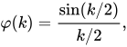
Viewing the rectangular function as a probability density function, it is a special case of the continuous uniform distribution with $a=-1/2,b=1/2.$ The characteristic function is

$\varphi (k)={\frac {\sin(k/2)}{k/2}},$

and its moment-generating function is

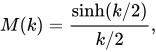
$M(k)={\frac {\sinh(k/2)}{k/2}},$

where $\sinh(t)$ is the hyperbolic sine function.

06Rational approximation

The pulse function may also be expressed as a limit of a rational function:

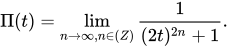
$\Pi (t)=\lim _{n\rightarrow \infty ,n\in \mathbb {(} Z)}{\frac {1}{(2t)^{2n}+1}}.$

07Dirac delta function

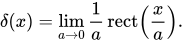
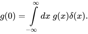
The rectangle function can be used to represent the Dirac delta function $\delta (x)$ . Specifically, $\delta (x)=\lim _{a\to 0}{\frac {1}{a}}\operatorname {rect} \left({\frac {x}{a}}\right).$ For a function $g(x)$ , its average over the width $a$ around 0 in the function domain is calculated as,

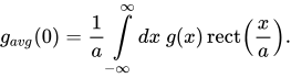
$g_{avg}(0)={\frac {1}{a}}\int \limits _{-\infty }^{\infty }dx\ g(x)\operatorname {rect} \left({\frac {x}{a}}\right).$ To obtain $g(0)$ , the following limit is applied,

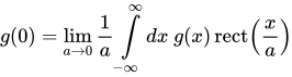
$g(0)=\lim _{a\to 0}{\frac {1}{a}}\int \limits _{-\infty }^{\infty }dx\ g(x)\operatorname {rect} \left({\frac {x}{a}}\right)$ and this can be written in terms of the Dirac delta function as, $g(0)=\int \limits _{-\infty }^{\infty }dx\ g(x)\delta (x).$ The Fourier transform of the Dirac delta function $\delta (t)$ is

$\delta (f)=\int _{-\infty }^{\infty }\delta (t)\cdot e^{-i2\pi ft}\,dt=\lim _{a\to 0}{\frac {1}{a}}\int _{-\infty }^{\infty }\operatorname {rect} \left({\frac {t}{a}}\right)\cdot e^{-i2\pi ft}\,dt=\lim _{a\to 0}\operatorname {sinc} {(af)}.$ where the sinc function here is the normalized sinc function. Because the first zero of the sinc function is at $f=1/a$ and $a$ goes to infinity, the Fourier transform of $\delta (t)$ is

$\delta (f)=1,$ means that the frequency spectrum of the Dirac delta function is infinitely broad. As a pulse is shorten in time, it is larger in spectrum.

Watch videos about Rectangular functionExplainers and documentaries on YouTube (opens in a new tab)

Sources and credits

This article is adapted from the Wikipedia article “Rectangular function”, written by its contributors and licensed under CC BY-SA 4.0. Fathomly has changed the layout, removed citation markers, navigation and maintenance notices, and adjusted punctuation. This adapted version is shared under the same license. For references, see the original article.

Images, from Wikimedia Commons:

Rectangular function.svg by Unknown author, CC BY-SA 3.0
Sinc function (normalized).svg by Omegatron, CC BY-SA 3.0
Splines resulting from successive convolution of the unit Rect function.png by Green Montanan, CC0

Fathomly is not affiliated with or endorsed by the Wikimedia Foundation. Spotted a problem? Tell us.

Rectangular function

01History

02Relation to the boxcar function

03Fourier transform of the rectangular function

04Self convolution of the Rectangular function

05Use in probability

06Rational approximation

07Dirac delta function

Sources and credits

Related topics

Fourier transform

Square wave (waveform)

Step function