Encyclopedia

Flow-based generative model

Statistical model used in machine learning

Wikipedia contributorsAdapted for Fathomly · View authors

16 min read
Source updated August 15, 2026

A flow-based generative model is a generative model used in machine learning that explicitly models a probability distribution by leveraging normalizing flow, which is a statistical method using the change-of-variable law of probabilities to transform a simple distribution into a complex one.

The direct modeling of likelihood provides many advantages. For example, the negative log-likelihood can be directly computed and minimized as the loss function. Additionally, novel samples can be generated by sampling from the initial distribution, and applying the flow transformation.

In contrast, many alternative generative modeling methods, such as variational autoencoders (VAEs), generative adversarial networks (GANs), or diffusion models, do not explicitly represent the likelihood function.

01Method

Let $z_{0}$ be a (possibly multivariate) random variable with distribution $p_{0}(z_{0})$ .

For $i=1,...,K$ , let $z_{i}=f_{i}(z_{i-1})$ be a sequence of random variables transformed from $z_{0}$ . The functions $f_{1},...,f_{K}$ should be invertible, i.e. the inverse function $f_{i}^{-1}$ exists. The final output $z_{K}$ models the target distribution.

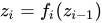
The log likelihood of $z_{K}$ is (see derivation):

$\log p_{K}(z_{K})=\log p_{0}(z_{0})-\sum _{i=1}^{K}\log \left|\det {\frac {df_{i}(z_{i-1})}{dz_{i-1}}}\right|$

Learning probability distributions by differentiating such log Jacobians originated in the Infomax (maximum likelihood) approach to ICA, which forms a single-layer (K=1) flow-based model. Relatedly, the single layer precursor of conditional generative flows appeared in.

To efficiently compute the log likelihood, the functions $f_{1},...,f_{K}$ should be easily invertible, and the determinants of their Jacobians should be simple to compute. In practice, the functions $f_{1},...,f_{K}$ are modeled using deep neural networks, and are trained to minimize the negative log-likelihood of data samples from the target distribution. These architectures are usually designed such that only the forward pass of the neural network is required in both the inverse and the Jacobian determinant calculations. Examples of such architectures include NICE, RealNVP, and Glow.

Derivation of log likelihood

Consider $z_{1}$ and $z_{0}$ . Note that $z_{0}=f_{1}^{-1}(z_{1})$ .

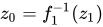
By the change of variable formula, the distribution of $z_{1}$ is:

$p_{1}(z_{1})=p_{0}(z_{0})\left|\det {\frac {df_{1}^{-1}(z_{1})}{dz_{1}}}\right|$

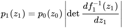
Where 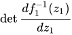$\det {\frac {df_{1}^{-1}(z_{1})}{dz_{1}}}$ is the determinant of the Jacobian matrix of $f_{1}^{-1}$ .

By the inverse function theorem:

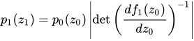
$p_{1}(z_{1})=p_{0}(z_{0})\left|\det \left({\frac {df_{1}(z_{0})}{dz_{0}}}\right)^{-1}\right|$

By the identity $\det(A^{-1})=\det(A)^{-1}$ (where $A$ is an invertible matrix), we have:

$p_{1}(z_{1})=p_{0}(z_{0})\left|\det {\frac {df_{1}(z_{0})}{dz_{0}}}\right|^{-1}$

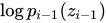
The log likelihood is thus:

$\log p_{1}(z_{1})=\log p_{0}(z_{0})-\log \left|\det {\frac {df_{1}(z_{0})}{dz_{0}}}\right|$

In general, the above applies to any $z_{i}$ and $z_{i-1}$ . Since $\log p_{i}(z_{i})$ is equal to $\log p_{i-1}(z_{i-1})$ subtracted by a non-recursive term, we can infer by induction that:

$\log p_{K}(z_{K})=\log p_{0}(z_{0})-\sum _{i=1}^{K}\log \left|\det {\frac {df_{i}(z_{i-1})}{dz_{i-1}}}\right|$

02Training method

As is generally done when training a deep learning model, the goal with normalizing flows is to minimize the Kullback-Leibler divergence between the model's likelihood and the target distribution to be estimated. Denoting $p_{\theta }$ the model's likelihood and $p^{*}$ the target distribution to learn, the (forward) KL-divergence is:

$D_{\text{KL}}[p^{*}(x)\|p_{\theta }(x)]=-\mathop {\mathbb {E} } _{p^{*}(x)}[\log p_{\theta }(x)]+\mathop {\mathbb {E} } _{p^{*}(x)}[\log p^{*}(x)]$

The second term on the right-hand side of the equation corresponds to the entropy of the target distribution and is independent of the parameter $\theta$ we want the model to learn, which only leaves the expectation of the negative log-likelihood to minimize under the target distribution. This intractable term can be approximated with a Monte-Carlo method by importance sampling. Indeed, if we have a dataset $\{x_{i}\}_{i=1}^{N}$ of samples each independently drawn from the target distribution $p^{*}(x)$ , then this term can be estimated as:

$-{\hat {\mathop {\mathbb {E} } }}_{p^{*}(x)}[\log p_{\theta }(x)]=-{\frac {1}{N}}\sum _{i=0}^{N}\log p_{\theta }(x_{i})$

Therefore, the learning objective

${\underset {\theta }{\operatorname {arg\,min} }}\ D_{\text{KL}}[p^{*}(x)\|p_{\theta }(x)]$

is replaced by

${\underset {\theta }{\operatorname {arg\,max} }}\ \sum _{i=0}^{N}\log p_{\theta }(x_{i})$

In other words, minimizing the Kullback-Leibler divergence between the model's likelihood and the target distribution is equivalent to maximizing the model likelihood under observed samples of the target distribution.

A pseudocode for training normalizing flows is as follows:

INPUT. dataset $x_{1:n}$ , normalizing flow model $f_{\theta }(\cdot ),p_{0}$ .
SOLVE. $\max _{\theta }\sum _{j}\log p_{\theta }(x_{j})$ by gradient descent
RETURN. ${\hat {\theta }}$

03Variants

Planar Flow

The earliest example. Fix some activation function $h$ , and let $\theta =(u,w,b)$ with the appropriate dimensions, then $x=f_{\theta }(z)=z+uh(\langle w,z\rangle +b)$ The inverse $f_{\theta }^{-1}$ has no closed-form solution in general.

The Jacobian is $|\det(I+h'(\langle w,z\rangle +b)uw^{T})|=|1+h'(\langle w,z\rangle +b)\langle u,w\rangle |$ .

For it to be invertible everywhere, it must be nonzero everywhere. For example, $h=\tanh$ and $\langle u,w\rangle >-1$ satisfies the requirement.

Nonlinear Independent Components Estimation (NICE)

Let $x,z\in \mathbb {R} ^{2n}$ be even-dimensional, and split them in the middle. Then the normalizing flow functions are $x={\begin{bmatrix}x_{1}\\x_{2}\end{bmatrix}}=f_{\theta }(z)={\begin{bmatrix}z_{1}\\z_{2}\end{bmatrix}}+{\begin{bmatrix}0\\m_{\theta }(z_{1})\end{bmatrix}}$ where $m_{\theta }$ is any neural network with weights $\theta$ .

$f_{\theta }^{-1}$ is just $z_{1}=x_{1},z_{2}=x_{2}-m_{\theta }(x_{1})$ , and the Jacobian is just 1, that is, the flow is volume-preserving.

When $n=1$ , this is seen as a curvy shearing along the $x_{2}$ direction.

Real Non-Volume Preserving (Real NVP)

The Real Non-Volume Preserving model generalizes NICE model by: $x={\begin{bmatrix}x_{1}\\x_{2}\end{bmatrix}}=f_{\theta }(z)={\begin{bmatrix}z_{1}\\e^{s_{\theta }(z_{1})}\odot z_{2}\end{bmatrix}}+{\begin{bmatrix}0\\m_{\theta }(z_{1})\end{bmatrix}}$

Its inverse is $z_{1}=x_{1},z_{2}=e^{-s_{\theta }(x_{1})}\odot (x_{2}-m_{\theta }(x_{1}))$ , and its Jacobian is $\prod _{i=1}^{n}e^{s_{\theta }(z_{1,})}$ . The NICE model is recovered by setting $s_{\theta }=0$ . Since the Real NVP map keeps the first and second halves of the vector $x$ separate, it's usually required to add a permutation $(x_{1},x_{2})\mapsto (x_{2},x_{1})$ after every Real NVP layer.

Generative Flow (Glow)

In generative flow model, each layer has 3 parts:

channel-wise affine transform $y_{cij}=s_{c}(x_{cij}+b_{c})$ with Jacobian $\prod _{c}s_{c}^{HW}$ .
invertible 1x1 convolution $z_{cij}=\sum _{c'}K_{cc'}y_{cij}$ with Jacobian $\det(K)^{HW}$ . Here $K$ is any invertible matrix.
Real NVP, with Jacobian as described in Real NVP.

The idea of using the invertible 1x1 convolution is to permute all layers in general, instead of merely permuting the first and second half, as in Real NVP.

Masked Autoregressive Flow (MAF)

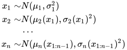
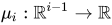
An autoregressive model of a distribution on $\mathbb {R} ^{n}$ is defined as the following stochastic process:

${\begin{aligned}x_{1}\sim &N(\mu _{1},\sigma _{1}^{2})\\x_{2}\sim &N(\mu _{2}(x_{1}),\sigma _{2}(x_{1})^{2})\\&\cdots \\x_{n}\sim &N(\mu _{n}(x_{1:n-1}),\sigma _{n}(x_{1:n-1})^{2})\\\end{aligned}}$ where $\mu _{i}:\mathbb {R} ^{i-1}\to \mathbb {R}$ and $\sigma _{i}:\mathbb {R} ^{i-1}\to (0,\infty )$ are fixed functions that define the autoregressive model.

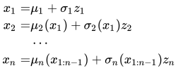
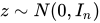
By the reparameterization trick, the autoregressive model is generalized to a normalizing flow: ${\begin{aligned}x_{1}=&\mu _{1}+\sigma _{1}z_{1}\\x_{2}=&\mu _{2}(x_{1})+\sigma _{2}(x_{1})z_{2}\\&\cdots \\x_{n}=&\mu _{n}(x_{1:n-1})+\sigma _{n}(x_{1:n-1})z_{n}\\\end{aligned}}$ The autoregressive model is recovered by setting $z\sim N(0,I_{n})$ .

The forward mapping is slow (because it's sequential), but the backward mapping is fast (because it's parallel).

The Jacobian matrix is lower-diagonal, so the Jacobian is $\sigma _{1}\sigma _{2}(x_{1})\cdots \sigma _{n}(x_{1:n-1})$ .

Reversing the two maps $f_{\theta }$ and $f_{\theta }^{-1}$ of MAF results in Inverse Autoregressive Flow (IAF), which has fast forward mapping and slow backward mapping.

Continuous Normalizing Flow (CNF)

Instead of constructing flow by function composition, another approach is to formulate the flow as a continuous-time dynamic. Let $z_{0}$ be the latent variable with distribution $p(z_{0})$ . Map this latent variable to data space with the following flow function:

$x=F(z_{0})=z_{T}=z_{0}+\int _{0}^{T}f(z_{t},t)dt$

where $f$ is an arbitrary function and can be modeled with e.g. neural networks.

The inverse function is then naturally:

$z_{0}=F^{-1}(x)=z_{T}+\int _{T}^{0}f(z_{t},t)dt=z_{T}-\int _{0}^{T}f(z_{t},t)dt$

And the log-likelihood of $x$ can be found as:

$\log(p(x))=\log(p(z_{0}))-\int _{0}^{T}{\text{Tr}}\left[{\frac {\partial f}{\partial z_{t}}}\right]dt$

Since the trace depends only on the diagonal of the Jacobian $\partial _{z_{t}}f$ , this allows "free-form" Jacobian. Here, "free-form" means that there is no restriction on the Jacobian's form. It is contrasted with previous discrete models of normalizing flow, where the Jacobian is carefully designed to be only upper- or lower-diagonal, so that the Jacobian can be evaluated efficiently.

The trace can be estimated by "Hutchinson's trick":

Given any matrix $W\in \mathbb {R} ^{n\times n}$ , and any random $u\in \mathbb {R} ^{n}$ with $E[uu^{T}]=I$ , we have $E[u^{T}Wu]=tr(W)$ . (Proof: expand the expectation directly.)

Usually, the random vector is sampled from $N(0,I)$ (normal distribution) or $\{\pm n^{-1/2}\}^{n}$ (Rademacher distribution).

When $f$ is implemented as a neural network, neural ODE methods would be needed. Indeed, CNF was first proposed in the same paper that proposed neural ODE.

There are two main deficiencies of CNF, one is that a continuous flow must be a homeomorphism, thus preserve orientation and ambient isotopy (for example, it's impossible to flip a left-hand to a right-hand by continuous deforming of space, and it's impossible to turn a sphere inside out, or undo a knot), and the other is that the learned flow $f$ might be ill-behaved, due to degeneracy (that is, there are an infinite number of possible $f$ that all solve the same problem).

By adding extra dimensions, the CNF gains enough freedom to reverse orientation and go beyond ambient isotopy (just like how one can pick up a polygon from a desk and flip it around in 3-space, or unknot a knot in 4-space), yielding the "augmented neural ODE".

Any homeomorphism of $\mathbb {R} ^{n}$ can be approximated by a neural ODE operating on $\mathbb {R} ^{2n+1}$ , proved by combining Whitney embedding theorem for manifolds and the universal approximation theorem for neural networks.

To regularize the flow $f$ , one can impose regularization losses. The paper proposed the following regularization loss based on optimal transport theory: $\lambda _{K}\int _{0}^{T}\left\|f(z_{t},t)\right\|^{2}dt+\lambda _{J}\int _{0}^{T}\left\|\nabla _{z}f(z_{t},t)\right\|_{F}^{2}dt$ where $\lambda _{K},\lambda _{J}>0$ are hyperparameters. The first term punishes the model for oscillating the flow field over time, and the second term punishes it for oscillating the flow field over space. Both terms together guide the model into a flow that is smooth (not "bumpy") over space and time.

04Flows on manifolds

When a probabilistic flow transforms a distribution on an $m$ -dimensional smooth manifold embedded in $\mathbb {R} ^{n}$ , where $m<n$ , and where the transformation is specified as a function, $\mathbb {R} ^{n}\to \mathbb {R} ^{n}$ , the scaling factor between the source and transformed PDFs is not given by the naive computation of the determinant of the $n{\text{-by-}}n$ Jacobian (which is zero), but instead by the determinant(s) of one or more suitably defined $m{\text{-by-}}m$ matrices. This section is an interpretation of the tutorial in the appendix of Sorrenson et al.(2023), where the more general case of non-isometrically embedded Riemann manifolds is also treated. Here we restrict attention to isometrically embedded manifolds.

As running examples of manifolds with smooth, isometric embedding in $\mathbb {R} ^{n}$ we shall use:

The unit hypersphere: $\mathbb {S} ^{n-1}=\{\mathbf {x} \in \mathbb {R} ^{n}:\mathbf {x} '\mathbf {x} =1\}$ , where flows can be used to generalize e.g. Von Mises-Fisher or uniform spherical distributions.
The simplex interior: $\Delta ^{n-1}=\{\mathbf {p} =(p_{1},\dots ,p_{n})\in \mathbb {R} ^{n}:p_{i}>0,\sum _{i}p_{i}=1\}$ , where $n$ -way categorical distributions live; and where flows can be used to generalize e.g. Dirichlet, or uniform simplex distributions.

As a first example of a spherical manifold flow transform, consider the normalized linear transform, which radially projects onto the unit sphere the output of an invertible linear transform, parametrized by the $n{\text{-by-}}n$ invertible matrix $\mathbf {M}$ :

$f_{\text{lin}}(\mathbf {x} ;\mathbf {M} )={\frac {\mathbf {Mx} }{\lVert \mathbf {Mx} \rVert }}$

In full Euclidean space, $f_{\text{lin}}:\mathbb {R} ^{n}\to \mathbb {R} ^{n}$ is not invertible, but if we restrict the domain and co-domain to the unit sphere, then $f_{\text{lin}}:\mathbb {S} ^{n-1}\to \mathbb {S} ^{n-1}$ is invertible (more specifically it is a bijection and a homeomorphism and a diffeomorphism), with inverse $f_{\text{lin}}(\cdot \,;\mathbf {M} ^{-1})$ . The Jacobian of $f_{\text{lin}}:\mathbb {R} ^{n}\to \mathbb {R} ^{n}$ , at $\mathbf {y} =f_{\text{lin}}(\mathbf {x} ;\mathbf {M} )$ is $\lVert \mathbf {Mx} \rVert ^{-1}(\mathbf {I} _{n}-\mathbf {yy} ')\mathbf {M}$ , which has rank $n-1$ and determinant of zero; while as explained here, the factor (see subsection below) relating source and transformed densities is: $\lVert \mathbf {Mx} \rVert ^{-n}\left|\operatorname {det} \mathbf {M} \right|$ .

Differential volume ratio

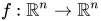
For $m<n$ , let ${\mathcal {M}}\subset \mathbb {R} ^{n}$ be an $m$ -dimensional manifold with a smooth, isometric embedding into $\mathbb {R} ^{n}$ . Let $f:\mathbb {R} ^{n}\to \mathbb {R} ^{n}$ be a smooth flow transform with range restricted to ${\mathcal {M}}$ . Let $\mathbf {x} \in {\mathcal {M}}$ be sampled from a distribution with density $P_{X}$ . Let $\mathbf {y} =f(\mathbf {x} )$ , with resultant (pushforward) density $P_{Y}$ . Let $U\subset {\mathcal {M}}$ be a small, convex region containing $\mathbf {x}$ and let $V=f(U)$ be its image, which contains $\mathbf {y}$ ; then by conservation of probability mass:

$P_{X}(\mathbf {x} )\operatorname {volume} (U)\approx P_{Y}(\mathbf {y} )\operatorname {volume} (V)$

where volume (for very small regions) is given by Lebesgue measure in $m$ -dimensional tangent space. By making the regions infinitessimally small, the factor relating the two densities is the ratio of volumes, which we term the differential volume ratio.

To obtain concrete formulas for volume on the $m$ -dimensional manifold, we construct $U$ by mapping an $m$ -dimensional rectangle in (local) coordinate space to the manifold via a smooth embedding function: $\mathbb {R} ^{m}\to \mathbb {R} ^{n}$ . At very small scale, the embedding function becomes essentially linear so that $U$ is a parallelotope (multidimensional generalization of a parallelogram). Similarly, the flow transform, $f$ becomes linear, so that the image, $V=f(U)$ is also a parallelotope. In $\mathbb {R} ^{m}$ , we can represent an $m$ -dimensional parallelotope with an $m{\text{-by-}}m$ matrix whose column-vectors are a set of edges (meeting at a common vertex) that span the paralellotope. The volume is given by the absolute value of the determinant of this matrix. If more generally (as is the case here), an $m$ -dimensional paralellotope is embedded in $\mathbb {R} ^{n}$ , it can be represented with a (tall) $n{\text{-by-}}m$ matrix, say $\mathbf {V}$ . Denoting the parallelotope as $/\mathbf {V} \!/$ , its volume is then given by the square root of the Gram determinant:

$\operatorname {volume} /\mathbf {V} \!/={\sqrt {\left|\operatorname {det} (\mathbf {V} '\mathbf {V} )\right|}}$

In the sections below, we show various ways to use this volume formula to derive the differential volume ratio.

Simplex flow

As a first example, we develop expressions for the differential volume ratio of a simplex flow, $\mathbf {q} =f(\mathbf {p} )$ , where $\mathbf {p} ,\mathbf {q} \in {\mathcal {M}}=\Delta ^{n-1}$ . Define the embedding function:

$e:{\tilde {\mathbf {p} }}=(p_{1}\dots ,p_{n-1})\mapsto \mathbf {p} =(p_{1}\dots ,p_{n-1},1-\sum _{i=1}^{n-1}p_{i})$

which maps a conveniently chosen, $(n-1)$ -dimensional representation, ${\tilde {\mathbf {p} }}$ , to the embedded manifold. The $n{\text{-by-}}(n-1)$ Jacobian is $\mathbf {E} ={\begin{bmatrix}\mathbf {I} _{n-1}\\-{\boldsymbol {1}}'\end{bmatrix}}$ . To define $U$ , the differential volume element at the transformation input ( $\mathbf {p} \in \Delta ^{n-1}$ ), we start with a rectangle in ${\tilde {\mathbf {p} }}$ -space, having (signed) differential side-lengths, $dp_{1},\dots ,dp_{n-1}$ from which we form the square diagonal matrix $\mathbf {D}$ , the columns of which span the rectangle. At very small scale, we get $U=e(\mathbf {D} )=/\mathbf {ED} \!/$ , with:

$\operatorname {volume} (U)={\sqrt {\left|\operatorname {det} (\mathbf {DE} '\mathbf {ED} )\right|}}={\sqrt {\left|\operatorname {det} (\mathbf {E} '\mathbf {E} )\right|}}\,\left|\operatorname {det} \mathbf {D} )\right|={\sqrt {n}}\prod _{i=1}^{n-1}\left|dp_{i}\right|$

To understand the geometric interpretation of the factor ${\sqrt {n}}$ , see the example for the 1-simplex in the diagram at right.

The differential volume element at the transformation output ( $\mathbf {q} \in \Delta ^{n-1}$ ), is the parallelotope, $V=f(U)=/\mathbf {F_{p}ED} \!/$ , where $\mathbf {F_{p}}$ is the $n{\text{-by-}}n$ Jacobian of $f$ at $\mathbf {p} =e({\tilde {\mathbf {p} }})$ . Its volume is:

$\operatorname {volume} (V)={\sqrt {\left|\operatorname {det} (\mathbf {DE} '\mathbf {F_{p}} '\mathbf {F_{p}ED} )\right|}}={\sqrt {\left|\operatorname {det} (\mathbf {E} '\mathbf {F_{p}} '\mathbf {F_{p}E} )\right|}}\,\left|\operatorname {det} \mathbf {D} )\right|$

so that the factor $\left|\operatorname {det} \mathbf {D} )\right|$ cancels in the volume ratio, which can now already be numerically evaluated. It can however be rewritten in a sometimes more convenient form by also introducing the representation function, $r:\mathbf {p} \mapsto {\tilde {\mathbf {p} }}$ , which simply extracts the first $(n-1)$ components. The Jacobian is $\mathbf {R} ={\begin{bmatrix}\mathbf {I} _{n}&{\boldsymbol {0}}\end{bmatrix}}$ . Observe that, since $e\circ r\circ f=f$ , the chain rule for function composition gives: $\mathbf {ERF_{p}} =\mathbf {F_{p}}$ . By plugging this expansion into the above Gram determinant and then refactoring it as a product of determinants of square matrices, we can extract the factor ${\sqrt {\left|\operatorname {det} (\mathbf {E} '\mathbf {E} )\right|}}={\sqrt {n}}$ , which now also cancels in the ratio, which finally simpifies to the determinant of the Jacobian of the "sandwiched" flow transformation, $r\circ f\circ e$ :

$R_{f}^{\Delta }(\mathbf {p} )={\frac {\operatorname {volume} (V)}{\operatorname {volume} (U)}}=\left|\operatorname {det} (\mathbf {RF_{p}E} )\right|$

which, if $\mathbf {p} \sim P_{\mathbf {P} }$ , can be used to derive the pushforward density after a change of variables, $\mathbf {q} =f(\mathbf {p} )$ :

$P_{\mathbf {Q} }(\mathbf {q} )={\frac {P_{\mathbf {P} }(\mathbf {p} )}{R_{f}^{\Delta }(\mathbf {p} )}}\,,\;{\text{where}}\;\;\mathbf {p} =f^{-1}(\mathbf {q} )$

This formula is valid only because the simplex is flat and the Jacobian, $\mathbf {E}$ is constant. The more general case for curved manifolds is discussed below, after we present two concrete examples of simplex flow transforms.

Simplex calibration transform

A calibration transform, $f_{\text{cal}}:\Delta ^{n-1}\to \Delta ^{n-1}$ , which is sometimes used in machine learning for post-processing of the (class posterior) outputs of a probabilistic $n$ -class classifier, uses the softmax function to renormalize categorical distributions after scaling and translation of the input distributions in log-probability space. For $\mathbf {p} ,\mathbf {q} \in \Delta ^{n-1}$ and with parameters, $a\neq 0$ and $\mathbf {c} \in \mathbb {R} ^{n}$ the transform can be specified as:

$\mathbf {q} =f_{\text{cal}}(\mathbf {p} ;a,\mathbf {c} )=\operatorname {softmax} (a^{-1}\log \mathbf {p} +\mathbf {c} )\;\iff \;\mathbf {p} =f_{\text{cal}}^{-1}(\mathbf {q} ;a,\mathbf {c} )=\operatorname {softmax} (a\log \mathbf {q} -a\mathbf {c} )$

where the log is applied elementwise. After some algebra the differential volume ratio can be expressed as:

$R_{\text{cal}}^{\Delta }(\mathbf {p} ;a,\mathbf {c} )=\left|\operatorname {det} (\mathbf {RF_{p}E} )\right|=\left|a\right|^{1-n}\prod _{i=1}^{n}{\frac {q_{i}}{p_{i}}}$

This result can also be obtained by factoring the density of the SGB distribution, which is obtained by sending Dirichlet variates through $f_{\text{cal}}$ .

While calibration transforms are most often trained as discriminative models, the reinterpretation here as a probabilistic flow allows also the design of generative calibration models based on this transform. When used for calibration, the restriction $a>0$ can be imposed to prevent direction reversal in log-probability space. With the additional restriction $\mathbf {c} ={\boldsymbol {0}}$ , this transform (with discriminative training) is known in machine learning as temperature scaling.

Generalized calibration transform

The above calibration transform can be generalized to $f_{\text{gcal}}:\Delta ^{n-1}\to \Delta ^{n-1}$ , with parameters $\mathbf {c} \in \mathbb {R} ^{n}$ and $\mathbf {A}$ $n{\text{-by-}}n$ invertible:

$\mathbf {q} =f_{\text{gcal}}(\mathbf {p} ;\mathbf {A} ,\mathbf {c} )=\operatorname {softmax} (\mathbf {A} \log \mathbf {p} +\mathbf {c} )\,,\;{\text{subject to}}\;\mathbf {A1} =\lambda \mathbf {1}$

where the condition that $\mathbf {A}$ has $\mathbf {1}$ as an eigenvector ensures invertibility by sidestepping the information loss due to the invariance: $\operatorname {softmax} (\mathbf {x} +\alpha \mathbf {1} )=\operatorname {softmax} (\mathbf {x} )$ . Note in particular that $\mathbf {A} =\lambda \mathbf {I} _{n}$ is the only allowed diagonal parametrization, in which case we recover $f_{\text{cal}}(\mathbf {p} ;\lambda ^{-1},\mathbf {c} )$ , while (for $n>2$ ) generalization is possible with non-diagonal matrices. The inverse is:

$\mathbf {p} =f_{\text{gcal}}^{-1}(\mathbf {q} ;\mathbf {A} ,\mathbf {c} )=f_{\text{gcal}}(\mathbf {q} ;\mathbf {A} ^{-1},-\mathbf {A} ^{-1}\mathbf {c} )\,,\;{\text{where}}\;\mathbf {A1} =\lambda \mathbf {1} \Longrightarrow \mathbf {A} ^{-1}\mathbf {1} =\lambda ^{-1}\mathbf {1}$

The differential volume ratio is:

$R_{\text{gcal}}^{\Delta }(\mathbf {p} ;\mathbf {A} ,\mathbf {c} )={\frac {\left|\operatorname {det} (\mathbf {A} )\right|}{|\lambda |}}\prod _{i=1}^{n}{\frac {q_{i}}{p_{i}}}$

If $f_{\text{gcal}}$ is to be used as a calibration transform, further constraint could be imposed, for example that $\mathbf {A}$ be positive definite, so that $(\mathbf {Ax} )'\mathbf {x} >0$ , which avoids direction reversals. (This is one possible generalization of $a>0$ in the $f_{\text{cal}}$ parameter.)

For $n=2$ , $a>0$ and $\mathbf {A}$ positive definite, then $f_{\text{cal}}$ and $f_{\text{gcal}}$ are equivalent in the sense that in both cases, $\log {\frac {p_{1}}{p_{2}}}\mapsto \log {\frac {q_{1}}{q_{2}}}$ is a straight line, the (positive) slope and offset of which are functions of the transform parameters. For $n>2,$ $f_{\text{gcal}}$ does generalize $f_{\text{cal}}$ .

It must however be noted that chaining multiple $f_{\text{gcal}}$ flow transformations does not give a further generalization, because:

$f_{\text{gcal}}(\cdot \,;\mathbf {A} _{1},\mathbf {c} _{1})\circ f_{\text{gcal}}(\cdot \,;\mathbf {A} _{2},\mathbf {c} _{2})=f_{\text{gcal}}(\cdot \,;\mathbf {A} _{1}\mathbf {A} _{2},\mathbf {c} _{1}+\mathbf {A} _{1}\mathbf {c} _{2})$

In fact, the set of $f_{\text{gcal}}$ transformations form a group under function composition. The set of $f_{\text{cal}}$ transformations form a subgroup.

Also see: Dirichlet calibration, which generalizes $f_{\text{gcal}}$ , by not placing any restriction on the matrix, $\mathbf {A}$ , so that invertibility is not guaranteed. While Dirichlet calibration is trained as a discriminative model, $f_{\text{gcal}}$ can also be trained as part of a generative calibration model.

Differential volume ratio for curved manifolds

Consider a flow, $\mathbf {y} =f(\mathbf {x} )$ on a curved manifold, for example $\mathbb {S} ^{n-1}$ which we equip with the embedding function, $e$ that maps a set of $(n-1)$ angular spherical coordinates to $\mathbb {S} ^{n-1}$ . The Jacobian of $e$ is non-constant and we have to evaluate it at both input ( $\mathbf {E_{x}}$ ) and output ( $\mathbf {E_{y}}$ ). The same applies to $r$ , the representation function that recovers spherical coordinates from points on $\mathbb {S} ^{n-1}$ , for which we need the Jacobian at the output ( $\mathbf {R_{y}}$ ). The differential volume ratio now generalizes to:

$R_{f}(\mathbf {x} )=\left|\operatorname {det} (\mathbf {R_{y}F_{x}E_{x}} )\right|\,{\frac {\sqrt {\left|\operatorname {det} (\mathbf {E} _{\mathbf {y} }'\mathbf {E_{y}} )\right|}}{\sqrt {\left|\operatorname {det} (\mathbf {E} _{\mathbf {x} }'\mathbf {E_{x}} )\right|}}}$

For geometric insight, consider $\mathbf {S} ^{2}$ , where the spherical coordinates are co-latitude, $\theta \in [0,\pi ]$ and longitude, $\phi \in [0,2\pi )$ . At $\mathbf {x} =e(\theta ,\phi )$ , we get ${\sqrt {\left|\operatorname {det} (\mathbf {E} _{\mathbf {x} }'\mathbf {E_{x}} )\right|}}=\sin \theta$ , which gives the radius of the circle at that latitude (compare e.g. polar circle to equator). The differential volume (surface area on the sphere) is: $\sin \theta \,d\theta \,d\phi$ .

The above derivation for $R_{f}$ is fragile in the sense that when using fixed functions $e,r$ , there may be places where they are not well-defined, for example at the poles of the 2-sphere where longitude is arbitrary. This problem is sidestepped (using standard manifold machinery) by generalizing to local coordinates (charts), where in the vicinities of $\mathbf {x} ,\mathbf {y} \in {\mathcal {M}}$ , we map from local $m$ -dimensional coordinates to $\mathbb {R} ^{n}$ and back using the respective function pairs $e_{\mathbf {x} },r_{\mathbf {x} }$ and $e_{\mathbf {y} },r_{\mathbf {y} }$ . We continue to use the same notation for the Jacobians of these functions ( $\mathbf {E_{x}} ,\mathbf {E_{y}} ,\mathbf {R_{y}}$ ), so that the above formula for $R_{f}$ remains valid.

We can however, choose our local coordinate system in a way that simplifies the expression for $R_{f}$ and indeed also its practical implementation. Let $\pi :{\mathcal {P}}\to \mathbb {R} ^{n}$ be a smooth idempotent projection ( $\pi \circ \pi =\pi$ ) from the projectible set, ${\mathcal {P}}\subseteq \mathbb {R} ^{n}$ , onto the embedded manifold. For example:

The positive orthant of $\mathbb {R} ^{n}$ is projected onto the simplex as: $\pi (\mathbf {z} )={\bigl (}\sum _{i=1}^{n}z_{i}{\bigr )}^{-1}\mathbf {z}$
Non-zero vectors in $\mathbb {R} ^{n}$ are projected onto the unit sphere as: $\pi (\mathbf {z} )={\bigl (}\sum _{i=1}^{n}z_{i}^{2}{\bigr )}^{-{\frac {1}{2}}}\mathbf {z}$

For every $\mathbf {x} \in {\mathcal {M}}$ , we require of $\pi$ that its $n{\text{-by-}}n$ Jacobian, ${\boldsymbol {\Pi _{x}}}$ has rank $m$ (the manifold dimension), in which case ${\boldsymbol {\Pi _{x}}}$ is an idempotent linear projection onto the local tangent space (orthogonal for the unit sphere: $\mathbf {I} _{n}-\mathbf {xx} '$ ; oblique for the simplex: $\mathbf {I} _{n}-{\boldsymbol {x1}}'$ ). The columns of ${\boldsymbol {\Pi _{x}}}$ span the $m$ -dimensional tangent space at $\mathbf {x}$ . We use the notation, $\mathbf {T_{x}}$ for any $n{\text{-by-}}m$ matrix with orthonormal columns ( $\mathbf {T} _{\mathbf {x} }'\mathbf {T_{x}} =\mathbf {I} _{m}$ ) that span the local tangent space. Also note: ${\boldsymbol {\Pi _{x}}}\mathbf {T_{x}} =\mathbf {T_{x}}$ . We can now choose our local coordinate embedding function, $e_{\mathbf {x} }:\mathbb {R} ^{m}\to \mathbb {R} ^{n}$ :

$e_{\mathbf {x} }({\tilde {x}})=\pi (\mathbf {x} +\mathbf {T_{x}{\tilde {x}}} )\,,{\text{with Jacobian:}}\,\mathbf {E_{x}} =\mathbf {T_{x}} \,{\text{at}}\,{\tilde {\mathbf {x} }}=\mathbf {0} .$

Since the Jacobian is injective (full rank: $m$ ), a local (not necessarily unique) left inverse, say $r_{\mathbf {x} }^{*}$ with Jacobian $\mathbf {R} _{\mathbf {x} }^{*}$ , exists such that $r_{\mathbf {x} }^{*}(e_{\mathbf {x} }({\tilde {x}}))={\tilde {x}}$ and $\mathbf {R} _{\mathbf {x} }^{*}\mathbf {T_{x}} =\mathbf {I} _{m}$ . In practice we do not need the left inverse function itself, but we do need its Jacobian, for which the above equation does not give a unique solution. We can however enforce a unique solution for the Jacobian by choosing the left inverse as, $r_{\mathbf {x} }:\mathbb {R} ^{n}\to \mathbb {R} ^{m}$ :

$r_{\mathbf {x} }(\mathbf {z} )=r_{\mathbf {x} }^{*}(\pi (\mathbf {z} ))\,,{\text{with Jacobian:}}\,\mathbf {R_{x}} =\mathbf {T} _{\mathbf {x} }'$

We can now finally plug $\mathbf {E_{x}} =\mathbf {T_{x}}$ and $\mathbf {R_{y}} =\mathbf {T} _{\mathbf {y} }'$ into our previous expression for $R_{f}$ , the differential volume ratio, which because of the orthonormal Jacobians, simplifies to:

$R_{f}(\mathbf {x} )=\left|\operatorname {det} (\mathbf {T_{y}} '\mathbf {F_{x}T_{x}} )\right|$

Practical implementation

For learning the parameters of a manifold flow transformation, we need access to the differential volume ratio, $R_{f}$ , or at least to its gradient w.r.t. the parameters. Moreover, for some inference tasks, we need access to $R_{f}$ itself. Practical solutions include:

Sorrenson et al.(2023) give a solution for computationally efficient stochastic parameter gradient approximation for $\log R_{f}.$
For some hand-designed flow transforms, $R_{f}$ can be analytically derived in closed form, for example the above-mentioned simplex calibration transforms. Further examples are given below in the section on simple spherical flows.
On a software platform equipped with linear algebra and automatic differentiation, $R_{f}(\mathbf {x} )=\left|\operatorname {det} (\mathbf {T_{y}} '\mathbf {F_{x}T_{x}} )\right|$ can be automatically evaluated, given access to only $\mathbf {x} ,f,\pi$ . But this is expensive for high-dimensional data, with at least ${\mathcal {O}}(n^{3})$ computational costs. Even then, the slow automatic solution can be invaluable as a tool for numerically verifying hand-designed closed-form solutions.

Simple spherical flows

In machine learning literature, various complex spherical flows formed by deep neural network architectures may be found. In contrast, this section compiles from statistics literature the details of three very simple spherical flow transforms, with simple closed-form expressions for inverses and differential volume ratios. These flows can be used individually, or chained, to generalize distributions on the unit sphere, $\mathbb {S} ^{n-1}$ . All three flows are compositions of an invertible affine transform in $\mathbb {R} ^{n}$ , followed by radial projection back onto the sphere. The flavours we consider for the affine transform are: pure translation, pure linear and general affine. To make these flows fully functional for learning, inference and sampling, the tasks are:

To derive the inverse transform, with suitable restrictions on the parameters to ensure invertibility.
To derive in simple closed form the differential volume ratio, $R_{f}$ .

An interesting property of these simple spherical flows is that they don't make use of any non-linearities apart from the radial projection. Even the simplest of them, the normalized translation flow, can be chained to form perhaps surprisingly flexible distributions.

Normalized translation flow

The normalized translation flow, $f_{\text{trans}}:\mathbb {S} ^{n-1}\to \mathbb {S} ^{n-1}$ , with parameter $\mathbf {c} \in \mathbb {R} ^{n}$ , is given by:

$\mathbf {y} =f_{\text{trans}}(\mathbf {x} ;\mathbf {c} )={\frac {\mathbf {x} +\mathbf {c} }{\lVert \mathbf {x} +\mathbf {c} \rVert }}\,,\;{\text{where}}\;\lVert \mathbf {c} \rVert <1$

The inverse function may be derived by considering, for $\ell >0$ : $\mathbf {y} =\ell ^{-1}(\mathbf {x} +\mathbf {c} )$ and then using $\mathbf {x} '\mathbf {x} =1$ to get a quadratic equation to recover $\ell$ , which gives:

$\mathbf {x} =f_{\text{trans}}^{-1}(\mathbf {y} ;\mathbf {c} )=\ell \mathbf {y} -\mathbf {c} \,,{\text{where}}\;\ell =\mathbf {y} '\mathbf {c} +{\sqrt {(\mathbf {y} '\mathbf {c} )^{2}+1-\mathbf {c} '\mathbf {c} }}$

from which we see that we need $\lVert \mathbf {c} \rVert <1$ to keep $\ell$ real and positive for all $\mathbf {y} \in \mathbb {S} ^{n-1}$ . The differential volume ratio is given (without derivation) by Boulerice & Ducharme(1994) as:

$R_{\text{trans}}(\mathbf {x} ;\mathbf {c} )={\frac {1+\mathbf {x} '\mathbf {c} }{\lVert \mathbf {x} +\mathbf {c} \rVert ^{n}}}$

This can indeed be verified analytically:

By a laborious manipulation of $R_{f}(\mathbf {x} )=\left|\operatorname {det} (\mathbf {T_{y}} '\mathbf {F_{x}T_{x}} )\right|$ .
By setting $\mathbf {M} =\mathbf {I} _{n}$ in $R_{\text{aff}}(\mathbf {x} ;\mathbf {M} ,\mathbf {c} )$ , which is given below.

Finally, it is worth noting that $f_{\text{trans}}$ and $f_{\text{trans}}^{-1}$ do not have the same functional form.

Normalized linear flow

The normalized linear flow, $f_{\text{lin}}:\mathbb {S} ^{n-1}\to \mathbb {S} ^{n-1}$ , where parameter $\mathbf {M}$ is an invertible $n{\text{-by-}}n$ matrix, is given by:

$\mathbf {y} =f_{\text{lin}}(\mathbf {x} ;\mathbf {M} )={\frac {\mathbf {Mx} }{\lVert \mathbf {Mx} \rVert }}\;\iff \;\mathbf {x} =f_{\text{lin}}^{-1}(\mathbf {y} ;\mathbf {M} )=f_{\text{lin}}(\mathbf {y} ;\mathbf {M} ^{-1})={\frac {\mathbf {M^{-1}y} }{\lVert \mathbf {M^{-1}y} \rVert }}$

The differential volume ratio is:

$R_{\text{lin}}(\mathbf {x} ;\mathbf {M} )={\frac {\left|\operatorname {det} \mathbf {M} \right|}{\lVert \mathbf {Mx} \rVert ^{n}}}$

This result can be derived indirectly via the Angular central Gaussian distribution (ACG), which can be obtained via normalized linear transform of either Gaussian, or uniform spherical variates. The first relationship can be used to derive the ACG density by a marginalization integral over the radius; after which the second relationship can be used to factor out the differential volume ratio. For details, see ACG distribution.

Normalized affine flow

The normalized affine flow, $f_{\text{aff}}:\mathbb {S} ^{n-1}\to \mathbb {S} ^{n-1}$ , with parameters $\mathbf {c} \in \mathbb {R} ^{n}$ and $\mathbf {M}$ , $n{\text{-by-}}n$ invertible, is given by:

$f_{\text{aff}}(\mathbf {x} ;\mathbf {M} ,\mathbf {c} )={\frac {\mathbf {Mx} +\mathbf {c} }{\lVert \mathbf {Mx} +\mathbf {c} \rVert }}\,,\;{\text{where}}\;\lVert \mathbf {M^{-1}c} \rVert <1$

The inverse function, derived in a similar way to the normalized translation inverse is:

$\mathbf {x} =f_{\text{aff}}^{-1}(\mathbf {y} ;\mathbf {M} ,\mathbf {c} )=\mathbf {M} ^{-1}(\ell \mathbf {y} -\mathbf {c} )\,,{\text{where}}\;\ell ={\frac {\mathbf {y} '\mathbf {Wc} +{\sqrt {(\mathbf {y} '\mathbf {Wc} )^{2}+\mathbf {y} '\mathbf {Wy} (1-\mathbf {c} '\mathbf {Wc} )}}}{\mathbf {y} '\mathbf {Wy} }}$

where $\mathbf {W} =(\mathbf {MM} ')^{-1}$ . The differential volume ratio is:

$R_{\text{aff}}(\mathbf {x} ;\mathbf {M} ,\mathbf {c} )=R_{\text{lin}}(\mathbf {x} ;\mathbf {M} +\mathbf {c} \mathbf {x} ')={\frac {\left|\operatorname {det} \mathbf {M} \right|(1+\mathbf {x} '\mathbf {M^{-1}c} )}{\lVert \mathbf {Mx+c} \rVert ^{n}}}$

The final RHS numerator was expanded from $\operatorname {det} (\mathbf {M} +\mathbf {cx} ')$ by the matrix determinant lemma. Recalling $R_{f}(\mathbf {x} )=\left|\operatorname {det} (\mathbf {T} _{\mathbf {y} }'\mathbf {F_{x}T_{x}} )\right|$ , the equality between $R_{\text{aff}}$ and $R_{\text{lin}}$ holds because not only:

$\mathbf {x} '\mathbf {x} =1\;\Longrightarrow \;\mathbf {y} =f_{\text{aff}}(\mathbf {x} ;\mathbf {M,c} )=f_{\text{lin}}(\mathbf {x} ;\mathbf {M+cx} ')$

but also, by orthogonality of $\mathbf {x}$ to the local tangent space:

$\mathbf {x} '\mathbf {T_{x}} ={\boldsymbol {0}}\;\Longrightarrow \;\mathbf {F} _{\mathbf {x} }^{\text{aff}}\mathbf {T_{x}} =\mathbf {F} _{\mathbf {x} }^{\text{lin}}\mathbf {T_{x}}$

where $\mathbf {F} _{\mathbf {x} }^{\text{lin}}=\lVert \mathbf {Mx} +\mathbf {c} \rVert ^{-1}(\mathbf {I} _{n}-\mathbf {yy} ')(\mathbf {M+cx} ')$ is the Jacobian of $f_{\text{lin}}$ differentiated w.r.t. its input, but not also w.r.t. its parameter.

05Downsides

Despite normalizing flows success in estimating high-dimensional densities, some downsides still exist in their designs. First of all, their latent space where input data is projected onto is not a lower-dimensional space and therefore, flow-based models do not allow for compression of data by default and require a lot of computation. However, it is still possible to perform image compression with them.

Flow-based models are also notorious for failing in estimating the likelihood of out-of-distribution samples (i.e.: samples that were not drawn from the same distribution as the training set). Some hypotheses were formulated to explain this phenomenon, among which the typical set hypothesis, estimation issues when training models, or fundamental issues due to the entropy of the data distributions.

One of the most interesting properties of normalizing flows is the invertibility of their learned bijective map. This property is given by constraints in the design of the models (cf.: RealNVP, Glow) which guarantee theoretical invertibility. The integrity of the inverse is important in order to ensure the applicability of the change-of-variable theorem, the computation of the Jacobian of the map as well as sampling with the model. However, in practice this invertibility is violated and the inverse map explodes because of numerical imprecision.

06Applications

Flow-based generative models have been applied on a variety of modeling tasks, including:

Audio generation
Image generation
Molecular graph generation
Point-cloud modeling
Video generation
Lossy image compression
Anomaly detection

Watch videos about Flow-based generative modelExplainers and documentaries on YouTube (opens in a new tab)

Sources and credits

This article is adapted from the Wikipedia article “Flow-based generative model”, written by its contributors and licensed under CC BY-SA 4.0. Fathomly has changed the layout, removed citation markers, navigation and maintenance notices, and adjusted punctuation. This adapted version is shared under the same license. For references, see the original article.

Images, from Wikimedia Commons:

Normalizing-flow.svg by https://github.com/janosh, MIT

Fathomly is not affiliated with or endorsed by the Wikimedia Foundation. Spotted a problem? Tell us.