Variational autoencoder
Deep learning generative model to encode data representation

In machine learning, a variational autoencoder (VAE) is an artificial neural network architecture introduced by Diederik P. Kingma and Max Welling in 2013. It is part of the families of probabilistic graphical models and variational Bayesian methods.
In addition to being seen as an autoencoder neural network architecture, variational autoencoders can also be studied within the mathematical formulation of variational Bayesian methods, connecting a neural encoder network to its decoder through a probabilistic latent space (for example, as a multivariate Gaussian distribution) that corresponds to the parameters of a variational distribution.
Thus, the encoder maps each point (such as an image) from a large complex dataset into a distribution within the latent space, rather than to a single point in that space. The decoder has the opposite function, which is to map from the latent space to the input space, again according to a distribution (although in practice, noise is rarely added during the decoding stage). By mapping a point to a distribution instead of a single point, the network can avoid overfitting the training data. Both networks are typically trained together with the usage of the reparameterization trick, although the variance of the noise model can be learned separately.
Although this type of model was initially designed for unsupervised learning, its effectiveness has been proven for semi-supervised learning and supervised learning.
01Overview of architecture and operation
A variational autoencoder is a generative model with a prior and noise distribution respectively. Usually such models are trained using the expectation-maximization meta-algorithm (e.g. probabilistic PCA, (spike & slab) sparse coding). Such a scheme optimizes a lower bound of the data likelihood, which is usually computationally intractable, and in doing so requires the discovery of q-distributions, or variational posteriors. These q-distributions are normally parameterized for each individual data point in a separate optimization process. However, variational autoencoders use a neural network as an amortized approach to jointly optimize across data points. In that way, the same parameters are reused for multiple data points, which can result in massive memory savings. The first neural network takes as input the data points themselves, and outputs parameters for the variational distribution. As it maps from a known input space to the low-dimensional latent space, it is called the encoder.
The decoder is the second neural network of this model. It is a function that maps from the latent space to the input space, e.g. as the means of the noise distribution. It is possible to use another neural network that maps to the variance, however this can be omitted for simplicity. In such a case, the variance can be optimized with gradient descent.
To optimize this model, one needs to know two terms: the "reconstruction error", and the Kullback-Leibler divergence (KL-D). Both terms are derived from the free energy expression of the probabilistic model, and therefore differ depending on the noise distribution and the assumed prior of the data, here referred to as p-distribution. For example, a standard VAE task such as IMAGENET is typically assumed to have a gaussianly distributed noise; however, tasks such as binarized MNIST require a Bernoulli noise. The KL-D from the free energy expression maximizes the probability mass of the q-distribution that overlaps with the p-distribution, which unfortunately can result in mode-seeking behaviour. The "reconstruction" term is the remainder of the free energy expression, and requires a sampling approximation to compute its expectation value.
More recent approaches replace Kullback-Leibler divergence (KL-D) with various statistical distances, see "Statistical distance VAE variants" below.

02Formulation
From the point of view of probabilistic modeling, one wants to maximize the likelihood of the data 



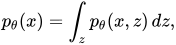
where 

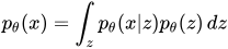
In the vanilla variational autoencoder, 
It is now possible to define the set of the relationships between the input data and its latent representation as
- Prior
- Likelihood
- Posterior
Unfortunately, the computation of 

with 


In this way, the problem is to find a good probabilistic autoencoder, in which the conditional likelihood distribution 

Parametrize the encoder as 

03Evidence lower bound (ELBO)
Like many deep learning approaches that use gradient-based optimization, VAEs require a differentiable loss function to update the network weights through backpropagation.
For variational autoencoders, the idea is to jointly optimize the generative model parameters 

The Kullback-Leibler divergence 
![{\begin{aligned}D_{KL}(q_{\phi }({z|x})\parallel p_{\theta }({z|x}))&=\mathbb {E} _{z\sim q_{\phi }(\cdot |x)}\left[\ln {\frac {q_{\phi }(z|x)}{p_{\theta }(z|x)}}\right]\\&=\mathbb {E} _{z\sim q_{\phi }(\cdot |x)}\left[\ln {\frac {q_{\phi }({z|x})p_{\theta }(x)}{p_{\theta }(x,z)}}\right]\\&=\ln p_{\theta }(x)+\mathbb {E} _{z\sim q_{\phi }(\cdot |x)}\left[\ln {\frac {q_{\phi }({z|x})}{p_{\theta }(x,z)}}\right].\end{aligned}}](https://wikimedia.org/api/rest_v1/media/math/render/svg/2c3333fd933e9a009a6474de60c63dabb9e88c0f)
Now, define the evidence lower bound (ELBO):![L_{\theta ,\phi }(x):=\mathbb {E} _{z\sim q_{\phi }(\cdot |x)}\left[\ln {\frac {p_{\theta }(x,z)}{q_{\phi }({z|x})}}\right]=\ln p_{\theta }(x)-D_{KL}(q_{\phi }({\cdot |x})\parallel p_{\theta }({\cdot |x}))](https://wikimedia.org/api/rest_v1/media/math/render/svg/f3930aaedee5df702f84e1571372c645eefa6572)
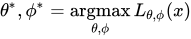


The form given is not very convenient for maximization, but the following, equivalent form, is:![L_{\theta ,\phi }(x)=\mathbb {E} _{z\sim q_{\phi }(\cdot |x)}\left[\ln p_{\theta }(x|z)\right]-D_{KL}(q_{\phi }({\cdot |x})\parallel p_{\theta }(\cdot ))](https://wikimedia.org/api/rest_v1/media/math/render/svg/e4ab2e155d237ffd569ef918817953a3ef82612c)

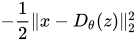




![L_{\theta ,\phi }(x)=-{\frac {1}{2}}\mathbb {E} _{z\sim q_{\phi }(\cdot |x)}\left[\|x-D_{\theta }(z)\|_{2}^{2}\right]-{\frac {1}{2}}\left(N\sigma _{\phi }(x)^{2}+\|E_{\phi }(x)\|_{2}^{2}-2N\ln \sigma _{\phi }(x)\right)+Const](https://wikimedia.org/api/rest_v1/media/math/render/svg/166eb4fc2e504a10271e5bad8ba9fd0f69bc6de5)

04Reparameterization
To efficiently search for
It is straightforward to find![\nabla _{\theta }\mathbb {E} _{z\sim q_{\phi }(\cdot |x)}\left[\ln {\frac {p_{\theta }(x,z)}{q_{\phi }({z|x})}}\right]=\mathbb {E} _{z\sim q_{\phi }(\cdot |x)}\left[\nabla _{\theta }\ln {\frac {p_{\theta }(x,z)}{q_{\phi }({z|x})}}\right]](https://wikimedia.org/api/rest_v1/media/math/render/svg/95305894e3cfbd10c985a9569091220891523aef)
![\nabla _{\phi }\mathbb {E} _{z\sim q_{\phi }(\cdot |x)}\left[\ln {\frac {p_{\theta }(x,z)}{q_{\phi }({z|x})}}\right]](https://wikimedia.org/api/rest_v1/media/math/render/svg/bd826d47c8a9e4ac5fc59cef9026f401e9806df6)

The most important example is when 

This can be reparametrized by letting 



![\nabla _{\phi }\mathbb {E} _{z\sim q_{\phi }(\cdot |x)}\left[\ln {\frac {p_{\theta }(x,z)}{q_{\phi }({z|x})}}\right]=\mathbb {E} _{\epsilon }\left[\nabla _{\phi }\ln {\frac {p_{\theta }(x,\mu _{\phi }(x)+L_{\phi }(x)\epsilon )}{q_{\phi }(\mu _{\phi }(x)+L_{\phi }(x)\epsilon |x)}}\right]](https://wikimedia.org/api/rest_v1/media/math/render/svg/ab3c8e4238659d4273a37de83c8c40ce58c789fb)
Since we reparametrized 





05Variations
Many variational autoencoders applications and extensions have been used to adapt the architecture to other domains and improve its performance.

The conditional VAE (CVAE), inserts label information in the latent space to force a deterministic constrained representation of the learned data.
Some structures directly deal with the quality of the generated samples or implement more than one latent space to further improve the representation learning.
Some architectures mix VAE and generative adversarial networks to obtain hybrid models.
It is not necessary to use gradients to update the encoder. In fact, the encoder is not necessary for the generative model.
06Statistical distance VAE variants
After the initial work of Diederik P. Kingma and Max Welling, several procedures were proposed to formulate in a more abstract way the operation of the VAE. In these approaches the loss function is composed of two parts:
- the usual reconstruction error part which seeks to ensure that the encoder-then-decoder mapping
is as close to the identity map as possible; the sampling is done at run time from the empirical distribution
of objects available (e.g., for MNIST or IMAGENET this will be the empirical probability law of all images in the dataset). This gives the term:
.
- a variational part that ensures that, when the empirical distribution
that is usually taken to be a Multivariate normal distribution. We will denote
this pushforward measure which in practice is just the empirical distribution obtained by passing all dataset objects through the encoder
is invoked and the term
is added to the loss.
We obtain the final formula for the loss:
![L_{\theta ,\phi }=\mathbb {E} _{x\sim \mathbb {P} ^{real}}\left[\|x-D_{\theta }(E_{\phi }(x))\|_{2}^{2}\right]+d\left(\mu (dz),E_{\phi }\sharp \mathbb {P} ^{real}\right)^{2}](https://wikimedia.org/api/rest_v1/media/math/render/svg/27e124b4786baa4f3b16d342cacb5889d032d44b)
The statistical distance
- the sliced Wasserstein distance used by S Kolouri, et al. in their VAE
- the energy distance implemented in the Radon Sobolev Variational Auto-Encoder
- the Maximum Mean Discrepancy distance used in the MMD-VAE
- the Wasserstein distance used in the WAEs
- kernel-based distances used in the Kernelized Variational Autoencoder (K-VAE)
Sources and credits
This article is adapted from the Wikipedia article “Variational autoencoder”, written by its contributors and licensed under CC BY-SA 4.0. Fathomly has changed the layout, removed citation markers, navigation and maintenance notices, and adjusted punctuation. This adapted version is shared under the same license. For references, see the original article.
Images, from Wikimedia Commons:
- VAE Basic.png by EugenioTL, CC BY-SA 4.0
- Reparameterization Trick.png by EugenioTL, CC BY-SA 4.0
- Reparameterized Variational Autoencoder.png by EugenioTL, CC BY-SA 4.0
Fathomly is not affiliated with or endorsed by the Wikimedia Foundation. Spotted a problem? Tell us.


