Encyclopedia

Inverse function theorem

Theorem in mathematics

Wikipedia contributorsAdapted for Fathomly · View authors

16 min read
Source updated September 9, 2026

In mathematical analysis, the inverse function theorem gives sufficient conditions for a function to have an inverse function. The essential idea is that if the best linear approximation to the function at a point is invertible, then with sufficient regularity assumptions, the function should also be invertible near that point. In its simplest form, the theorem states that if a real function f is differentiable in an open interval, with a continuous derivative, then in a neighborhood of any point where the derivative is not zero, f has an inverse function. The inverse function is also continuously differentiable, and the inverse function rule expresses its derivative as the multiplicative inverse of the derivative of f.

The theorem applies verbatim to complex-valued functions of a complex variable. It generalizes to functions from n-tuples (of real or complex numbers) to n-tuples, and to functions between vector spaces of the same finite dimension, by replacing "derivative" with "Jacobian matrix" and "nonzero derivative" with "nonzero Jacobian determinant".

If the function of the theorem belongs to a higher differentiability class, the same is true for the inverse function. There are also versions of the inverse function theorem for holomorphic functions, for differentiable maps between manifolds, for differentiable functions between Banach spaces, and so forth.

The theorem was first established by Picard and Goursat using an iterative scheme: the basic idea is to prove a fixed point theorem using the contraction mapping theorem.

01Statements

One variable

The inverse function theorem is not often stated separately for one variable, because a stronger result is true: if a real-valued function of a single real variable has a derivative which is nonzero on an interval, then the function has an inverse throughout the interval. More precisely, suppose that $f$ is a real-valued differentiable function on an open interval $I$ , and $f'$ is non-zero throughout $I$ . Then the image of the interval $I$ is another interval $J$ , $f:I\to J$ is a bijection, and has a differentiable inverse function $f^{-1}:J\to I$ . This theorem is true because the non-vanishing of the derivative implies that it must be entirely of one sign (positive or negative) according to Darboux's theorem, and therefore the function must be strictly monotone, and thus one-to-one.

The inverse function theorem is a weaker local statement. The statement of the inverse function theorem is, roughly speaking, that if a real-valued function $f$ of a single real variable has a continuous derivative on an open interval $I$ , then it is locally invertible near each point where its derivative is non-zero. More precisely, around any point $x$ in $I$ where $f'(x)\neq 0$ , there is a smaller interval $I'$ on which the function $f$ is one-to-one and the image of the interval $I'$ under $f$ is also an open interval $J'$ . Thus $f$ maps the interval $I'$ bijectively onto the interval $J'$ . The inverse function theorem in this form follows at once from the stronger global result, by restricting the interval $I$ to a smaller interval $I'$ around $x$ on which the derivative is non-zero throughout.

When $f$ is continuously differentiable, the inverse function $f^{-1}:J'\to I'$ is also continuously differentiable, and its derivative at any point $y$ in the interval $J'$ is given by the inverse function rule: ${\frac {d}{dy}}f^{-1}(y)={\frac {1}{f'(f^{-1}(y))}}.$

The derivative being non-zero at a point is a sufficient condition for the function to have a local inverse, but it is not necessary. A function $f$ may be injective near a point $a$ while $f'(a)=0$ . An example is $f(x)=(x-a)^{3}$ . But, for such a function, the inverse cannot be differentiable at $b=f(a)$ , since if $f^{-1}$ were differentiable at $b$ , then, by the chain rule, $1=(f^{-1}\circ f)'(a)=(f^{-1})'(b)f'(a)$ , which implies $f'(a)\neq 0$ . (The situation is different for holomorphic functions; see Holomorphic inverse function theorem below.)

Several variables

For functions of more than one variable, the theorem states that if $f$ is a continuously differentiable function from an open subset $A$ of $\mathbb {R} ^{n}$ into $\mathbb {R} ^{n}$ , and the derivative $f'(a)$ is invertible at a point a (that is, the determinant of the Jacobian matrix of f at a is non-zero), then there exist open neighborhoods $U$ of $a$ in $A$ and $V$ of $b=f(a)$ such that $f(U)=V$ and $f:U\to V$ is bijective. Writing $f=(f_{1},\ldots ,f_{n})$ , this means that the system of n equations $y_{i}=f_{i}(x_{1},\dots ,x_{n})$ has a unique solution for $x_{1},\dots ,x_{n}$ in terms of $y_{1},\dots ,y_{n}$ when $x\in U,y\in V$ . Note that, unlike the case of a single variable, the theorem does not say $f$ is bijective onto the image where $f'$ is invertible but that it is locally bijective where $f'$ is invertible.

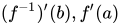
Moreover, the theorem says that the inverse function $f^{-1}:V\to U$ is continuously differentiable, and its derivative at $b=f(a)$ is the inverse map of $f'(a)$ ; i.e.,

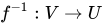
$(f^{-1})'(b)=f'(a)^{-1}.$

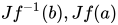
In other words, if $Jf^{-1}(b),Jf(a)$ are the Jacobian matrices representing $(f^{-1})'(b),f'(a)$ , this means:

$Jf^{-1}(b)=Jf(a)^{-1}.$

The hard part in this formula is the existence and differentiability of $f^{-1}$ . Assuming this, the inverse derivative formula follows from the chain rule applied to $f^{-1}\circ f=I$ . (Indeed, $1=I'(a)=(f^{-1}\circ f)'(a)=(f^{-1})'(b)\circ f'(a).$ ) Since taking the inverse is infinitely differentiable, the formula for the derivative of the inverse shows that if $f$ is continuously $k$ times differentiable, with invertible derivative at the point a, then the inverse is also continuously $k$ times differentiable. Here $k$ is a positive integer or $\infty$ .

There are two variants of the inverse function theorem. Given a continuously differentiable map $f:U\to \mathbb {R} ^{m}$ , the first is

The derivative $f'(a)$ is surjective (i.e., the Jacobian matrix representing it has rank $m$ ) if and only if there exists a continuously differentiable function $g$ on a neighborhood $V$ of $b=f(a)$ such that $f\circ g=I$ near $b$ ,

and the second is

The derivative $f'(a)$ is injective if and only if there exists a continuously differentiable function $g$ on a neighborhood $V$ of $b=f(a)$ such that $g\circ f=I$ near $a$ .

In the first case (when $f'(a)$ is surjective), the point $b=f(a)$ is called a regular value. Since $m=\dim \ker(f'(a))+\dim \operatorname {im} (f'(a))$ , the first case is equivalent to saying $b=f(a)$ is not in the image of critical points $a$ (a critical point is a point $a$ such that the kernel of $f'(a)$ is nonzero). The statement in the first case is a special case of the submersion theorem.

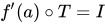
These variants are restatements of the inverse functions theorem. Indeed, in the first case when $f'(a)$ is surjective, we can find an (injective) linear map $T$ such that $f'(a)\circ T=I$ . Define $h(x)=a+Tx$ so that we have:

$(f\circ h)'(0)=f'(a)\circ T=I.$

Thus, by the inverse function theorem, $f\circ h$ has inverse near $0$ ; i.e., $f\circ h\circ (f\circ h)^{-1}=I$ near $b$ . The second case ( $f'(a)$ is injective) is seen in the similar way.

The function is bounded inside a quadratic envelope near the line , so . Nevertheless, it has local max/min points accumulating at , so it is not one-to-one on any surrounding interval.

02Example

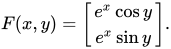
Consider the vector-valued function $F:\mathbb {R} ^{2}\to \mathbb {R} ^{2}\!$ defined by:

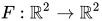
$F(x,y)={\begin{bmatrix}{e^{x}\cos y}\\{e^{x}\sin y}\\\end{bmatrix}}.$

The Jacobian matrix of it at $(x,y)$ is:

$JF(x,y)={\begin{bmatrix}{e^{x}\cos y}&{-e^{x}\sin y}\\{e^{x}\sin y}&{e^{x}\cos y}\\\end{bmatrix}}$

with the determinant:

$\det JF(x,y)=e^{2x}\cos ^{2}y+e^{2x}\sin ^{2}y=e^{2x}.\,\!$

The determinant $e^{2x}\!$ is nonzero everywhere. Thus the theorem guarantees that, for every point p in $\mathbb {R} ^{2}\!$ , there exists a neighborhood about p over which F is invertible. This does not mean F is invertible over its entire domain: in this case F is not even injective since it is periodic: $F(x,y)=F(x,y+2\pi )\!$ .

03Counter-example

If one drops the assumption that the derivative is continuous, the function is no longer necessarily locally injective. For example $f(x)=x+2x^{2}\sin({\tfrac {1}{x}})$ and $f(0)=0$ has discontinuous derivative $f'\!(x)=1-2\cos({\tfrac {1}{x}})+4x\sin({\tfrac {1}{x}})$ and $f'\!(0)=1,$ which vanishes arbitrarily close to $x=0$ . These critical points are local max/min points of $f,$ so $f$ is not one-to-one (and not invertible) on any interval containing $x=0$ . Intuitively, the slope $f'\!(0)=1$ does not propagate to nearby points, where the slopes rapidly oscillate between -1 and 3 (approximately).

If the derivative is continuous but zero at a point, the function is no longer necessarily locally injective. A real function that is locally constant at a point $x\in \mathbb {R}$ in the interior of its domain is not locally injective at $x$ but is trivially continuously differentiable at $x$ .

04Methods of proof

As an important result, the inverse function theorem has been given numerous proofs. The proof most commonly seen in textbooks relies on the contraction mapping principle, also known as the Banach fixed-point theorem (which can also be used as the key step in the proof of existence and uniqueness of solutions to ordinary differential equations).

Since the fixed point theorem applies in infinite-dimensional (Banach space) settings, this proof generalizes immediately to the infinite-dimensional version of the inverse function theorem (see Generalizations below).

An alternate proof in finite dimensions hinges on the extreme value theorem for functions on a compact set. This approach has an advantage that the proof generalizes to a situation where there is no Cauchy completeness (see § Over a real closed field).

Yet another proof uses Newton's method, which has the advantage of providing an effective version of the theorem: bounds on the derivative of the function imply an estimate of the size of the neighborhood on which the function is invertible.

Proof for single-variable functions

We want to prove the following: Let $D\subseteq \mathbb {R}$ be an open set with $x_{0}\in D,f:D\to \mathbb {R}$ a continuously differentiable function defined on $D$ , and suppose that $f'(x_{0})\neq 0$ . Then there exists an open interval $I$ with $x_{0}\in I$ such that $f$ maps $I$ bijectively onto the open interval $J=f(I)$ , and such that the inverse function $f^{-1}:J\to I$ is continuously differentiable, and for any $y\in J$ , if $x\in I$ is such that $f(x)=y$ , then $(f^{-1})'(y)={\dfrac {1}{f'(x)}}$ .

We may without loss of generality assume that $f'(x_{0})>0$ . Given that $D$ is an open set and $f'$ is continuous at $x_{0}$ , there exists $r>0$ such that $(x_{0}-r,x_{0}+r)\subseteq D$ and $|f'(x)-f'(x_{0})|<{\dfrac {f'(x_{0})}{2}}\qquad {\text{for all }}|x-x_{0}|<r.$

In particular, $f'(x)>{\dfrac {f'(x_{0})}{2}}>0\qquad {\text{for all }}|x-x_{0}|<r.$

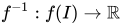
This shows that $f$ is strictly increasing for all $|x-x_{0}|<r$ . Let $\delta >0$ be such that $\delta <r$ . Then $[x-\delta ,x+\delta ]\subseteq (x_{0}-r,x_{0}+r)$ . By the intermediate value theorem, we find that $f$ maps the interval $[x-\delta ,x+\delta ]$ bijectively onto $[f(x-\delta ),f(x+\delta )]$ . Denote by $I=(x-\delta ,x+\delta )$ and $J=(f(x-\delta ),f(x+\delta ))$ . Then $f:I\to J$ is a bijection and the inverse $f^{-1}:J\to I$ exists. The fact that $f^{-1}:J\to I$ is differentiable follows from the differentiability of $f$ . In particular, the result follows from the fact that if $f:I\to \mathbb {R}$ is a strictly monotonic and continuous function that is differentiable at $x_{0}\in I$ with $f'(x_{0})\neq 0$ , then $f^{-1}:f(I)\to \mathbb {R}$ is differentiable with $(f^{-1})'(y_{0})={\dfrac {1}{f'(x_{0})}}$ , where $y_{0}=f(x_{0})$ (a standard result in analysis). This completes the proof.

A proof using successive approximation

To prove existence, it can be assumed after an affine transformation that $f(0)=0$ and $f^{\prime }(0)=I$ , so that $a=b=0$ .

By the mean value theorem for vector-valued functions, for a differentiable function $u:[0,1]\to \mathbb {R} ^{m}$ , ${\textstyle \|u(1)-u(0)\|\leq \sup _{0\leq t\leq 1}\|u^{\prime }(t)\|$ . Setting $u(t)=f(x+t(x^{\prime }-x))-x-t(x^{\prime }-x)$ , it follows that

$\|f(x)-f(x^{\prime })-x+x^{\prime }\|\leq \|x-x^{\prime }\|\,\sup _{0\leq t\leq 1}\|f^{\prime }(x+t(x^{\prime }-x))-I\|.$

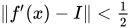
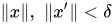
Now choose $\delta >0$ so that ${\textstyle \|f'(x)-I\|<{1 \over 2}$ for $\|x\|<\delta$ . Suppose that $\|y\|<\delta /2$ and define $x_{n}$ inductively by $x_{0}=0$ and $x_{n+1}=x_{n}+y-f(x_{n})$ . The assumptions show that if $\|x\|,\,\,\|x^{\prime }\|<\delta$ then

$\|f(x)-f(x^{\prime })-x+x^{\prime }\|\leq \|x-x^{\prime }\|/2$ .

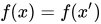
In particular $f(x)=f(x^{\prime })$ implies $x=x^{\prime }$ . In the inductive scheme $\|x_{n}\|<\delta$ and $\|x_{n+1}-x_{n}\|<\delta /2^{n}$ . Thus $(x_{n})$ is a Cauchy sequence tending to $x$ . By construction $f(x)=y$ as required.

To check that $g=f^{-1}$ is C¹, write $g(y+k)=x+h$ so that $f(x+h)=f(x)+k$ . By the inequalities above, $\|h-k\|<\|h\|/2$ so that $\|h\|/2<\|k\|<2\|h\|$ . On the other hand, if $A=f^{\prime }(x)$ , then $\|A-I\|<1/2$ . Using the geometric series for $B=I-A$ , it follows that $\|A^{-1}\|<2$ . But then

${\|g(y+k)-g(y)-f^{\prime }(g(y))^{-1}k\| \over \|k\|}={\|h-f^{\prime }(x)^{-1}[f(x+h)-f(x)]\| \over \|k\|}\leq 4{\|f(x+h)-f(x)-f^{\prime }(x)h\| \over \|h\|}$

tends to 0 as $k$ and $h$ tend to 0, proving that $g$ is C¹ with $g^{\prime }(y)=f^{\prime }(g(y))^{-1}$ .

The proof above is presented for a finite-dimensional space, but applies equally well for Banach spaces. If an invertible function $f$ is C^k with $k>1$ , then so too is its inverse. This follows by induction using the fact that the map $F(A)=A^{-1}$ on operators is C^k for any $k$ (in the finite-dimensional case this is an elementary fact because the inverse of a matrix is given as the adjugate matrix divided by its determinant). The method of proof here can be found in the books of Henri Cartan, Jean Dieudonné, Serge Lang, Roger Godement and Lars Hörmander.

A proof using the contraction mapping principle

Here is a proof based on the contraction mapping theorem. Specifically, following T. Tao, it uses the following consequence of the contraction mapping theorem.

Lemma, Let $B(0,r)$ denote an open ball of radius r in $\mathbb {R} ^{n}$ with center 0 and $g:B(0,r)\to \mathbb {R} ^{n}$ a map with a constant $0<c<1$ such that

$|g(y)-g(x)|\leq c|y-x|$

for all $x,y$ in $B(0,r)$ . Then for $f=I+g$ on $B(0,r)$ , we have

$(1-c)|x-y|\leq |f(x)-f(y)|,$

in particular, f is injective. If, moreover, $g(0)=0$ , then

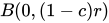
$B(0,(1-c)r)\subset f(B(0,r))\subset B(0,(1+c)r)$ .

More generally, the statement remains true if $\mathbb {R} ^{n}$ is replaced by a Banach space. Also, the first part of the lemma is true for any normed space.

Basically, the lemma says that a small perturbation of the identity map by a contraction map is injective and preserves a ball in some sense. Assuming the lemma for a moment, we prove the theorem first. As in the above proof, it is enough to prove the special case when $a=0,b=f(a)=0$ and $f'(0)=I$ . Let $g=f-I$ . The mean value inequality applied to $t\mapsto g(x+t(y-x))$ says:

$|g(y)-g(x)|\leq |y-x|\sup _{0<t<1}|g'(x+t(y-x))|.$

Since $g'(0)=I-I=0$ and $g'$ is continuous, we can find an $r>0$ such that

$|g(y)-g(x)|\leq 2^{-1}|y-x|$

for all $x,y$ in $B(0,r)$ . Then the early lemma says that $f=g+I$ is injective on $B(0,r)$ and $B(0,r/2)\subset f(B(0,r))$ . Then

$f:U=B(0,r)\cap f^{-1}(B(0,r/2))\to V=B(0,r/2)$

is bijective and thus has an inverse. Next, we show the inverse $f^{-1}$ is continuously differentiable (this part of the argument is the same as that in the previous proof). This time, let $g=f^{-1}$ denote the inverse of $f$ and $A=f'(x)$ . For $x=g(y)$ , we write $g(y+k)=x+h$ or $y+k=f(x+h)$ . Now, by the early estimate, we have

$|h-k|=|f(x+h)-f(x)-h|\leq |h|/2$

and so $|h|/2\leq |k|$ . Writing $\|\cdot \|$ for the operator norm,

$|g(y+k)-g(y)-A^{-1}k|=|h-A^{-1}(f(x+h)-f(x))|\leq \|A^{-1}\||Ah-f(x+h)+f(x)|.$

As $k\to 0$ , we have $h\to 0$ and $|h|/|k|$ is bounded. Hence, $g$ is differentiable at $y$ with the derivative $g'(y)=f'(g(y))^{-1}$ . Also, $g'$ is the same as the composition $\iota \circ f'\circ g$ where $\iota :T\mapsto T^{-1}$ ; so $g'$ is continuous.

It remains to show the lemma. First, we have:

$|x-y|-|f(x)-f(y)|\leq |g(x)-g(y)|\leq c|x-y|,$

which is to say

$(1-c)|x-y|\leq |f(x)-f(y)|.$

This proves the first part. Next, we show $f(B(0,r))\supset B(0,(1-c)r)$ . The idea is to note that this is equivalent to, given a point $y$ in $B(0,(1-c)r)$ , find a fixed point of the map

$F:{\overline {B}}(0,r')\to {\overline {B}}(0,r'),\,x\mapsto y-g(x)$

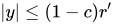
where $0<r'<r$ such that $|y|\leq (1-c)r'$ and the bar means a closed ball. To find a fixed point, we use the contraction mapping theorem and checking that $F$ is a well-defined strict-contraction mapping is straightforward. Finally, we have: $f(B(0,r))\subset B(0,(1+c)r)$ since

$|f(x)|=|x+g(x)-g(0)|\leq (1+c)|x|.\square$

As might be clear, this proof is not substantially different from the previous one, as the proof of the contraction mapping theorem is by successive approximation.

05Applications

Implicit function theorem

The inverse function theorem can be used to solve a system of equations

${\begin{aligned}&f_{1}(x)=y_{1}\\&\quad \vdots \\&f_{n}(x)=y_{n},\end{aligned}}$

i.e., expressing $y_{1},\dots ,y_{n}$ as functions of $x=(x_{1},\dots ,x_{n})$ , provided the Jacobian matrix is invertible. The implicit function theorem allows to solve a more general system of equations:

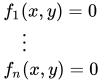
${\begin{aligned}&f_{1}(x,y)=0\\&\quad \vdots \\&f_{n}(x,y)=0\end{aligned}}$

for $y$ in terms of $x$ . Though more general, the theorem is actually a consequence of the inverse function theorem. First, the precise statement of the implicit function theorem is as follows:

given a map $f:\mathbb {R} ^{n}\times \mathbb {R} ^{m}\to \mathbb {R} ^{m}$ , if $f(a,b)=0$ , $f$ is continuously differentiable in a neighborhood of $(a,b)$ and the derivative of $y\mapsto f(a,y)$ at $b$ is invertible, then there exists a differentiable map $g:U\to V$ for some neighborhoods $U,V$ of $a,b$ such that $f(x,g(x))=0$ . Moreover, if $f(x,y)=0,x\in U,y\in V$ , then $y=g(x)$ ; i.e., $g(x)$ is a unique solution.

To see this, consider the map $F(x,y)=(x,f(x,y))$ . By the inverse function theorem, $F:U\times V\to W$ has the inverse $G$ for some neighborhoods $U,V,W$ . We then have:

$(x,y)=F(G_{1}(x,y),G_{2}(x,y))=(G_{1}(x,y),f(G_{1}(x,y),G_{2}(x,y))),$

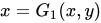
implying $x=G_{1}(x,y)$ and $y=f(x,G_{2}(x,y)).$ Thus $g(x)=G_{2}(x,0)$ has the required property. $\square$

Giving a manifold structure

In differential geometry, the inverse function theorem is used to show that the pre-image of a regular value under a smooth map is a manifold. Indeed, let $f:U\to \mathbb {R} ^{r}$ be such a smooth map from an open subset of $\mathbb {R} ^{n}$ (since the result is local, there is no loss of generality with considering such a map). Fix a point $a$ in $f^{-1}(b)$ and then, by permuting the coordinates on $\mathbb {R} ^{n}$ , assume the matrix $\left[{\frac {\partial f_{i}}{\partial x_{j}}}(a)\right]_{1\leq i,j\leq r}$ has rank $r$ . Then the map $F:U\to \mathbb {R} ^{r}\times \mathbb {R} ^{n-r}=\mathbb {R} ^{n},\,x\mapsto (f(x),x_{r+1},\dots ,x_{n})$ is such that $F'(a)$ has rank $n$ . Hence, by the inverse function theorem, we find the smooth inverse $G$ of $F$ defined in a neighborhood $V\times W$ of $(b,a_{r+1},\dots ,a_{n})$ . We then have

$x=(F\circ G)(x)=(f(G(x)),G_{r+1}(x),\dots ,G_{n}(x)),$

which implies

$(f\circ G)(x_{1},\dots ,x_{n})=(x_{1},\dots ,x_{r}).$

That is, after the change of coordinates by $G$ , $f$ is a coordinate projection (this fact is known as the submersion theorem). Moreover, since $G:V\times W\to U'=G(V\times W)$ is bijective, the map

$g=G(b,\cdot ):W\to f^{-1}(b)\cap U',\,(x_{r+1},\dots ,x_{n})\mapsto G(b,x_{r+1},\dots ,x_{n})$

is bijective with the smooth inverse. That is to say, $g$ gives a local parametrization of $f^{-1}(b)$ around $a$ . Hence, $f^{-1}(b)$ is a manifold. $\square$ (Note the proof is quite similar to the proof of the implicit function theorem and, in fact, the implicit function theorem can be also used instead.)

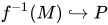
More generally, the theorem shows that if a smooth map $f:P\to E$ is transversal to a submanifold $M\subset E$ , then the pre-image $f^{-1}(M)\hookrightarrow P$ is a submanifold.

06Global version

The inverse function theorem is a local result; it applies to each point. A priori, the theorem thus only shows the function $f$ is locally bijective (or locally diffeomorphic of some class). The next topological lemma can be used to upgrade local injectivity to injectivity that is global to some extent.

Lemma, If $A$ is a closed subset of a (second-countable) topological manifold $X$ (or, more generally, a topological space admitting an exhaustion by compact subsets) and $f:X\to Z$ , $Z$ some topological space, is a local homeomorphism that is injective on $A$ , then $f$ is injective on some neighborhood of $A$ .

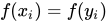
Proof: First assume $X$ is compact. If the conclusion of the theorem is false, we can find two sequences $x_{i}\neq y_{i}$ such that $f(x_{i})=f(y_{i})$ and $x_{i},y_{i}$ each converge to some points $x,y$ in $A$ . Since $f$ is injective on $A$ , $x=y$ . Now, if $i$ is large enough, $x_{i},y_{i}$ are in a neighborhood of $x=y$ where $f$ is injective; thus, $x_{i}=y_{i}$ , a contradiction.

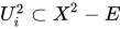
In general, consider the set $E=\{(x,y)\in X^{2}\mid x\neq y,f(x)=f(y)\}$ . It is disjoint from $S\times S$ for any subset $S\subset X$ where $f$ is injective. Let $X_{1}\subset X_{2}\subset \cdots$ be an increasing sequence of compact subsets with union $X$ and with $X_{i}$ contained in the interior of $X_{i+1}$ . Then, by the first part of the proof, for each $i$ , we can find a neighborhood $U_{i}$ of $A\cap X_{i}$ such that $U_{i}^{2}\subset X^{2}-E$ . Then $U=\bigcup _{i}U_{i}$ has the required property. $\square$ (See also for an alternative approach.)

The lemma implies the following (a sort of) global version of the inverse function theorem:

Inverse function theorem, Let $f:U\to V$ be a map between open subsets of $\mathbb {R} ^{n}$ or more generally of manifolds. Assume $f$ is continuously differentiable (or is $C^{k}$ ). If $f$ is injective on a closed subset $A\subset U$ and if the Jacobian matrix of $f$ is invertible at each point of $A$ , then $f$ is injective on a neighborhood $A'$ of $A$ and $f^{-1}:f(A')\to A'$ is continuously differentiable (or is $C^{k}$ ).

Note that if $A$ is a point, then the above is the usual inverse function theorem.

07Holomorphic inverse function theorem

There is a version of the inverse function theorem for holomorphic maps.

Theorem, Let $U,V\subset \mathbb {C} ^{n}$ be open subsets such that $0\in U$ and $f:U\to V$ a holomorphic map whose Jacobian matrix in variables $z_{i},{\overline {z}}_{i}$ is invertible (the determinant is nonzero) at $0$ . Then $f$ is injective in some neighborhood $W$ of $0$ and the inverse $f^{-1}:f(W)\to W$ is holomorphic.

The theorem follows from the usual inverse function theorem. Indeed, let $J_{\mathbb {R} }(f)$ denote the Jacobian matrix of $f$ in variables $x_{i},y_{i}$ and $J(f)$ for that in $z_{j},{\overline {z}}_{j}$ . Then we have $\det J_{\mathbb {R} }(f)=|\det J(f)|^{2}$ , which is nonzero by assumption. Hence, by the usual inverse function theorem, $f$ is injective near $0$ with continuously differentiable inverse. By chain rule, with $w=f(z)$ ,

${\frac {\partial }{\partial {\overline {z}}_{j}}}(f_{j}^{-1}\circ f)(z)=\sum _{k}{\frac {\partial f_{j}^{-1}}{\partial w_{k}}}(w){\frac {\partial f_{k}}{\partial {\overline {z}}_{j}}}(z)+\sum _{k}{\frac {\partial f_{j}^{-1}}{\partial {\overline {w}}_{k}}}(w){\frac {\partial {\overline {f}}_{k}}{\partial {\overline {z}}_{j}}}(z)$

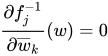
where the left-hand side and the first term on the right vanish since $f_{j}^{-1}\circ f$ and $f_{k}$ are holomorphic. Thus, ${\frac {\partial f_{j}^{-1}}{\partial {\overline {w}}_{k}}}(w)=0$ for each $k$ . $\square$

Similarly, there is the implicit function theorem for holomorphic functions.

As already noted earlier, it can happen that an injective smooth function has the inverse that is not smooth (e.g., $f(x)=x^{3}$ in a real variable). This is not the case for holomorphic functions because of:

Proposition, If $f:U\to V$ is an injective holomorphic map between open subsets of $\mathbb {C} ^{n}$ , then $f^{-1}:f(U)\to U$ is holomorphic.

08Formulations for manifolds

The inverse function theorem can be rephrased in terms of differentiable maps between differentiable manifolds. In this context the theorem states that for a differentiable map $F:M\to N$ (of class $C^{1}$ ), if the differential of $F$ ,

$dF_{p}:T_{p}M\to T_{F(p)}N$

is a linear isomorphism at a point $p$ in $M$ then there exists an open neighborhood $U$ of $p$ such that

$F|_{U}:U\to F(U)$

is a diffeomorphism. Note that this implies that the connected components of M and N containing p and F(p) have the same dimension, as is already directly implied from the assumption that dF_p is an isomorphism. If the derivative of F is an isomorphism at all points p in M then the map F is a local diffeomorphism.

09Banach spaces

The inverse function theorem can be generalized to differentiable maps between Banach spaces X and Y.

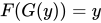
Let U be an open neighbourhood of the origin in X and $F:U\to Y\!$ a continuously differentiable function, and assume that the Fréchet derivative $dF_{0}:X\to Y\!$ of F at 0 is a bounded linear isomorphism of X onto Y. Then there exists an open neighbourhood V of $F(0)\!$ in Y and a continuously differentiable map $G:V\to X\!$ such that $F(G(y))=y$ for all y in V. Moreover, $G(y)\!$ is the only sufficiently small solution x of the equation $F(x)=y\!$ .

There is also the inverse function theorem for Banach manifolds.

Example

Consider the Banach spaces $X\subset C^{1}([0,1])$ of continuously-differentiable real-valued functions on the unit interval such that $f(0)=0$ , and $Y=C([0,1])$ of continuous functions on the unit interval. Define $F:X\to Y,\qquad F(u)=u'+u^{2}.$ Then ⁠ $F$ ⁠ is continuously Fréchet differentiable, and $DF(u)h=h'+2uh.$ At $u=0$ , the derivative is the operator ⁠ $h\mapsto h'$ ⁠. This is an isomorphism from ⁠ $X$ ⁠ to ⁠ $Y$ ⁠, with inverse $g\mapsto \left(t\mapsto \int _{0}^{t}g(s)\,ds\right).$ Therefore the inverse function theorem for Banach spaces implies that ⁠ $F$ ⁠ is locally invertible near ⁠ $0$ ⁠. In particular, for every sufficiently small ⁠ $g\in C([0,1])$ ⁠, the initial-value problem $u'(t)+u(t)^{2}=g(t),\qquad u(0)=0,$ has a unique small solution ⁠ $u\in C^{1}([0,1])$ ⁠, and this solution depends continuously differentiably on ⁠ $g$ ⁠.

10Generalizations

Constant rank theorem

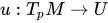
The inverse function theorem (and the implicit function theorem) can be seen as a special case of the constant rank theorem, which states that a smooth map with constant rank near a point can be put in a particular normal form near that point. Specifically, if $F:M\to N$ has constant rank near a point $p\in M\!$ , then there are open neighborhoods $U$ of $p$ and $V$ of $F(p)\!$ and there are diffeomorphisms $u:T_{p}M\to U\!$ and $v:T_{F(p)}N\to V\!$ such that $F(U)\subseteq V\!$ and such that the derivative $dF_{p}:T_{p}M\to T_{F(p)}N\!$ is equal to $v^{-1}\circ F\circ u.\!$ That is, $F$ "looks like" its derivative near $p$ . The set of points $p\in M$ such that the rank is constant in a neighborhood of $p$ is an open dense subset of $M$ ; this is a consequence of semicontinuity of the rank function. Thus the constant rank theorem applies to a generic point of the domain.

When the derivative of $F$ is injective (resp. surjective) at a point $p$ , it is also injective (resp. surjective) in a neighborhood of $p$ , and hence the rank of $F$ is constant on that neighborhood, and the constant rank theorem applies.

Polynomial functions

If it were true, the Jacobian conjecture would be a variant of the inverse function theorem for polynomials. It states that if a vector-valued polynomial function has a Jacobian determinant that is an invertible polynomial (that is a nonzero constant), then it has an inverse that is also a polynomial function. In July 2026, a counterexample has been provided that shows that the conjecture is false for three variables or more. For two variables, it remains unknown whether the conjecture is true or false. For a single variable, the conjecture is trivially true.

Selections

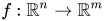
When $f:\mathbb {R} ^{n}\to \mathbb {R} ^{m}$ with $m\leq n$ , $f$ is $k$ times continuously differentiable, and the Jacobian $A=\nabla f({\overline {x}})$ at a point ${\overline {x}}$ is of rank $m$ , the inverse of $f$ may not be unique. However, there exists a local selection function $s$ such that $f(s(y))=y$ for all $y$ in a neighborhood of ${\overline {y}}=f({\overline {x}})$ , $s({\overline {y}})={\overline {x}}$ , $s$ is $k$ times continuously differentiable in this neighborhood, and $\nabla s({\overline {y}})=A^{T}(AA^{T})^{-1}$ ( $\nabla s({\overline {y}})$ is the Moore-Penrose pseudoinverse of $A$ ).

Over a real closed field

The inverse function theorem also holds over a real closed field k (or an o-minimal structure). Precisely, the theorem holds for a semialgebraic (or definable) map between open subsets of $k^{n}$ that is continuously differentiable.

The usual proof of the IFT uses Banach's fixed point theorem, which relies on the Cauchy completeness. That part of the argument is replaced by the use of the extreme value theorem, which does not need completeness. Explicitly, in § A proof using the contraction mapping principle, the Cauchy completeness is used only to establish the inclusion $B(0,r/2)\subset f(B(0,r))$ . Here, we shall directly show $B(0,r/4)\subset f(B(0,r))$ instead (which is enough). Given a point $y$ in $B(0,r/4)$ , consider the function $P(x)=|f(x)-y|^{2}$ defined on a neighborhood of ${\overline {B}}(0,r)$ . If $P'(x)=0$ , then $0=P'(x)=2[f_{1}(x)-y_{1}\cdots f_{n}(x)-y_{n}]f'(x)$ and so $f(x)=y$ , since $f'(x)$ is invertible. Now, by the extreme value theorem, $P$ admits a minimal at some point $x_{0}$ on the closed ball ${\overline {B}}(0,r)$ , which can be shown to lie in $B(0,r)$ using $2^{-1}|x|\leq |f(x)|$ . Since $P'(x_{0})=0$ , $f(x_{0})=y$ , which proves the claimed inclusion. $\square$

Alternatively, one can deduce the theorem from the one over real numbers by Tarski's principle.

Watch videos about Inverse function theoremExplainers and documentaries on YouTube (opens in a new tab)

Sources and credits

This article is adapted from the Wikipedia article “Inverse function theorem”, written by its contributors and licensed under CC BY-SA 4.0. Fathomly has changed the layout, removed citation markers, navigation and maintenance notices, and adjusted punctuation. This adapted version is shared under the same license. For references, see the original article.

Images, from Wikimedia Commons:

TangentGraphic2.svg by Chorch, Public domain
Inv-Fun-Thm-3.png by Magyar25, CC BY-SA 4.0

Fathomly is not affiliated with or endorsed by the Wikimedia Foundation. Spotted a problem? Tell us.