Multivariate analysis of variance
Procedure for comparing multivariate sample means

In statistics, multivariate analysis of variance (MANOVA) is a procedure for comparing multivariate sample means. As a multivariate procedure, it is used when there are two or more dependent variables, and is often followed by significance tests involving individual dependent variables separately.
Without relation to the image, the dependent variables may be k life satisfactions scores measured at sequential time points and p job satisfaction scores measured at sequential time points. In this case there are k+p dependent variables whose linear combination follows a multivariate normal distribution, multivariate variance-covariance matrix homogeneity, and linear relationship, no multicollinearity, and each without outliers.
01Model
Assume 








02Relationship with ANOVA
MANOVA is a generalized form of univariate analysis of variance (ANOVA), although, unlike univariate ANOVA, it uses the covariance between outcome variables in testing the statistical significance of the mean differences.
Where sums of squares appear in univariate analysis of variance, in multivariate analysis of variance certain positive-definite matrices appear. The diagonal entries are the same kinds of sums of squares that appear in univariate ANOVA. The off-diagonal entries are corresponding sums of products. Under normality assumptions about error distributions, the counterpart of the sum of squares due to error has a Wishart distribution.
03Hypothesis Testing
First, define the following 
: where the
: where the
. That is the mean over all observation in group
.
: where the

Then the matrix 



The most common statistics are summaries based on the roots (or eigenvalues) 

- Samuel Stanley Wilks'
distributed as lambda (Λ)
- the K. C. Sreedharan Pillai, M. S. Bartlett trace,
- the Lawley, Hotelling trace,
- Roy's greatest root (also called Roy's largest root),

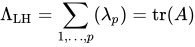

Discussion continues over the merits of each, although the greatest root leads only to a bound on significance which is not generally of practical interest. A further complication is that, except for the Roy's greatest root, the distribution of these statistics under the null hypothesis is not straightforward and can only be approximated except in a few low-dimensional cases. An algorithm for the distribution of the Roy's largest root under the null hypothesis was derived in while the distribution under the alternative is studied in.
The best-known approximation for Wilks' lambda was derived by C. R. Rao.
In the case of two groups, all the statistics are equivalent and the test reduces to Hotelling's T-square.

04Introducing covariates (MANCOVA)
One can also test if there is a group effect after adjusting for covariates. For this, follow the procedure above but substitute
Note that in case of unbalanced data, the order of adding the covariates matters.
05Correlation of dependent variables
MANOVA's power is affected by the correlations of the dependent variables and by the effect sizes associated with those variables. For example, when there are two groups and two dependent variables, MANOVA's power is lowest when the correlation equals the ratio of the smaller to the larger standardized effect size.
Sources and credits
This article is adapted from the Wikipedia article “Multivariate analysis of variance”, written by its contributors and licensed under CC BY-SA 4.0. Fathomly has changed the layout, removed citation markers, navigation and maintenance notices, and adjusted punctuation. This adapted version is shared under the same license. For references, see the original article.
Images, from Wikimedia Commons:
- Univariate vs. Multivariate.jpg by Unknown author, CC0
- Outcome Variables.jpg by Unknown author, CC0
- MANOVAs and Highly Correlated Dependent Variables.png by Manni2425, CC BY-SA 4.0
Fathomly is not affiliated with or endorsed by the Wikimedia Foundation. Spotted a problem? Tell us.
