Encyclopedia

Generalized eigenvector

Vector satisfying some of the criteria of an eigenvector

Wikipedia contributorsAdapted for Fathomly · View authors

11 min read
Source updated August 16, 2025

In linear algebra, a generalized eigenvector of an $n\times n$ matrix $A$ is a vector which satisfies certain criteria which are more relaxed than those for an (ordinary) eigenvector.

Let $V$ be an $n$ -dimensional vector space and let $A$ be the matrix representation of a linear map from $V$ to $V$ with respect to some ordered basis.

There may not always exist a full set of $n$ linearly independent eigenvectors of $A$ that form a complete basis for $V$ . That is, the matrix $A$ may not be diagonalizable. This happens when the algebraic multiplicity of at least one eigenvalue $\lambda _{i}$ is greater than its geometric multiplicity (the nullity of the matrix $(A-\lambda _{i}I)$ , or the dimension of its nullspace). In this case, $\lambda _{i}$ is called a defective eigenvalue and $A$ is called a defective matrix.

A generalized eigenvector $x_{i}$ corresponding to $\lambda _{i}$ , together with the matrix $(A-\lambda _{i}I)$ generate a Jordan chain of linearly independent generalized eigenvectors which form a basis for an invariant subspace of $V$ .

Using generalized eigenvectors, a set of linearly independent eigenvectors of $A$ can be extended, if necessary, to a complete basis for $V$ . This basis can be used to determine an "almost diagonal matrix" $J$ in Jordan normal form, similar to $A$ , which is useful in computing certain matrix functions of $A$ . The matrix $J$ is also useful in solving the system of linear differential equations $\mathbf {x} '=A\mathbf {x} ,$ where $A$ need not be diagonalizable.

The dimension of the generalized eigenspace corresponding to a given eigenvalue $\lambda$ is the algebraic multiplicity of $\lambda$ .

01Overview and definition

There are several equivalent ways to define an ordinary eigenvector. For our purposes, an eigenvector $\mathbf {u}$ associated with an eigenvalue $\lambda$ of an $n$ × $n$ matrix $A$ is a nonzero vector for which $(A-\lambda I)\mathbf {u} =\mathbf {0}$ , where $I$ is the $n$ × $n$ identity matrix and $\mathbf {0}$ is the zero vector of length $n$ . That is, $\mathbf {u}$ is in the kernel of the transformation $(A-\lambda I)$ . If $A$ has $n$ linearly independent eigenvectors, then $A$ is similar to a diagonal matrix $D$ . That is, there exists an invertible matrix $M$ such that $A$ is diagonalizable through the similarity transformation $D=M^{-1}AM$ . The matrix $D$ is called a spectral matrix for $A$ . The matrix $M$ is called a modal matrix for $A$ . Diagonalizable matrices are of particular interest since matrix functions of them can be computed easily.

On the other hand, if $A$ does not have $n$ linearly independent eigenvectors associated with it, then $A$ is not diagonalizable.

Definition: A vector $\mathbf {x} _{m}$ is a generalized eigenvector of rank m of the matrix $A$ and corresponding to the eigenvalue $\lambda$ if

$(A-\lambda I)^{m}\mathbf {x} _{m}=\mathbf {0}$

but

$(A-\lambda I)^{m-1}\mathbf {x} _{m}\neq \mathbf {0} .$

Clearly, a generalized eigenvector of rank 1 is an ordinary eigenvector. Every $n$ × $n$ matrix $A$ has $n$ linearly independent generalized eigenvectors associated with it and can be shown to be similar to an "almost diagonal" matrix $J$ in Jordan normal form. That is, there exists an invertible matrix $M$ such that $J=M^{-1}AM$ . The matrix $M$ in this case is called a generalized modal matrix for $A$ . If $\lambda$ is an eigenvalue of algebraic multiplicity $\mu$ , then $A$ will have $\mu$ linearly independent generalized eigenvectors corresponding to $\lambda$ . These results, in turn, provide a straightforward method for computing certain matrix functions of $A$ .

Note: For an $n\times n$ matrix $A$ over a field $F$ to be expressed in Jordan normal form, all eigenvalues of $A$ must be in $F$ . That is, the characteristic polynomial $f(x)$ must factor completely into linear factors; $F$ must be an algebraically closed field. For example, if $A$ has real-valued elements, then it may be necessary for the eigenvalues and the components of the eigenvectors to have complex values.

The set spanned by all generalized eigenvectors for a given $\lambda$ forms the generalized eigenspace for $\lambda$ .

02Examples

Here are some examples to illustrate the concept of generalized eigenvectors. Some of the details will be described later.

Example 1

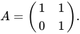
This example is simple but clearly illustrates the point. This type of matrix is used frequently in textbooks. Suppose

$A={\begin{pmatrix}1&1\\0&1\end{pmatrix}}.$

Then there is only one eigenvalue, $\lambda =1$ , and its algebraic multiplicity is $m=2$ .

Notice that this matrix is in Jordan normal form but is not diagonal. Hence, this matrix is not diagonalizable. Since there is one superdiagonal entry, there will be one generalized eigenvector of rank greater than 1 (or one could note that the vector space $V$ is of dimension 2, so there can be at most one generalized eigenvector of rank greater than 1). Alternatively, one could compute the dimension of the nullspace of $A-\lambda I$ to be $p=1$ , and thus there are $m-p=1$ generalized eigenvectors of rank greater than 1.

The ordinary eigenvector $\mathbf {v} _{1}={\begin{pmatrix}1\\0\end{pmatrix}}$ is computed as usual (see the eigenvector page for examples). Using this eigenvector, we compute the generalized eigenvector $\mathbf {v} _{2}$ by solving

$(A-\lambda I)\mathbf {v} _{2}=\mathbf {v} _{1}.$

Writing out the values:

$\left({\begin{pmatrix}1&1\\0&1\end{pmatrix}}-1{\begin{pmatrix}1&0\\0&1\end{pmatrix}}\right){\begin{pmatrix}v_{21}\\v_{22}\end{pmatrix}}={\begin{pmatrix}0&1\\0&0\end{pmatrix}}{\begin{pmatrix}v_{21}\\v_{22}\end{pmatrix}}={\begin{pmatrix}1\\0\end{pmatrix}}.$

This simplifies to

$v_{22}=1.$

The element $v_{21}$ has no restrictions. The generalized eigenvector of rank 2 is then $\mathbf {v} _{2}={\begin{pmatrix}a\\1\end{pmatrix}}$ , where a can have any scalar value. The choice of a = 0 is usually the simplest.

Note that

$(A-\lambda I)\mathbf {v} _{2}={\begin{pmatrix}0&1\\0&0\end{pmatrix}}{\begin{pmatrix}a\\1\end{pmatrix}}={\begin{pmatrix}1\\0\end{pmatrix}}=\mathbf {v} _{1},$

so that $\mathbf {v} _{2}$ is a generalized eigenvector, because

$(A-\lambda I)^{2}\mathbf {v} _{2}=(A-\lambda I)[(A-\lambda I)\mathbf {v} _{2}]=(A-\lambda I)\mathbf {v} _{1}={\begin{pmatrix}0&1\\0&0\end{pmatrix}}{\begin{pmatrix}1\\0\end{pmatrix}}={\begin{pmatrix}0\\0\end{pmatrix}}=\mathbf {0} ,$

so that $\mathbf {v} _{1}$ is an ordinary eigenvector, and that $\mathbf {v} _{1}$ and $\mathbf {v} _{2}$ are linearly independent and hence constitute a basis for the vector space $V$ .

Example 2

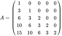
This example is more complex than Example 1. Unfortunately, it is a little difficult to construct an interesting example of low order. The matrix

$A={\begin{pmatrix}1&0&0&0&0\\3&1&0&0&0\\6&3&2&0&0\\10&6&3&2&0\\15&10&6&3&2\end{pmatrix}}$

has eigenvalues $\lambda _{1}=1$ and $\lambda _{2}=2$ with algebraic multiplicities $\mu _{1}=2$ and $\mu _{2}=3$ , but geometric multiplicities $\gamma _{1}=1$ and $\gamma _{2}=1$ .

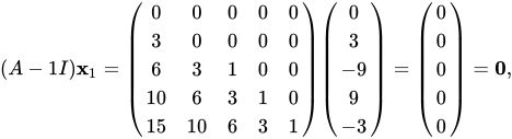
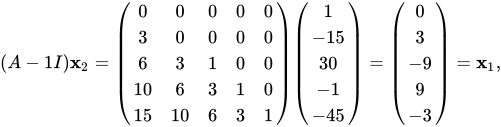
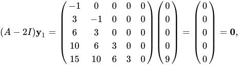
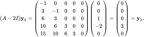
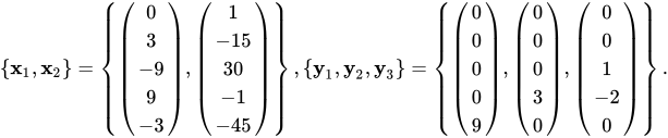
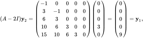
The generalized eigenspaces of $A$ are calculated below. $\mathbf {x} _{1}$ is the ordinary eigenvector associated with $\lambda _{1}$ . $\mathbf {x} _{2}$ is a generalized eigenvector associated with $\lambda _{1}$ . $\mathbf {y} _{1}$ is the ordinary eigenvector associated with $\lambda _{2}$ . $\mathbf {y} _{2}$ and $\mathbf {y} _{3}$ are generalized eigenvectors associated with $\lambda _{2}$ .

$(A-1I)\mathbf {x} _{1}={\begin{pmatrix}0&0&0&0&0\\3&0&0&0&0\\6&3&1&0&0\\10&6&3&1&0\\15&10&6&3&1\end{pmatrix}}{\begin{pmatrix}0\\3\\-9\\9\\-3\end{pmatrix}}={\begin{pmatrix}0\\0\\0\\0\\0\end{pmatrix}}=\mathbf {0} ,$

$(A-1I)\mathbf {x} _{2}={\begin{pmatrix}0&0&0&0&0\\3&0&0&0&0\\6&3&1&0&0\\10&6&3&1&0\\15&10&6&3&1\end{pmatrix}}{\begin{pmatrix}1\\-15\\30\\-1\\-45\end{pmatrix}}={\begin{pmatrix}0\\3\\-9\\9\\-3\end{pmatrix}}=\mathbf {x} _{1},$

$(A-2I)\mathbf {y} _{1}={\begin{pmatrix}-1&0&0&0&0\\3&-1&0&0&0\\6&3&0&0&0\\10&6&3&0&0\\15&10&6&3&0\end{pmatrix}}{\begin{pmatrix}0\\0\\0\\0\\9\end{pmatrix}}={\begin{pmatrix}0\\0\\0\\0\\0\end{pmatrix}}=\mathbf {0} ,$

$(A-2I)\mathbf {y} _{2}={\begin{pmatrix}-1&0&0&0&0\\3&-1&0&0&0\\6&3&0&0&0\\10&6&3&0&0\\15&10&6&3&0\end{pmatrix}}{\begin{pmatrix}0\\0\\0\\3\\0\end{pmatrix}}={\begin{pmatrix}0\\0\\0\\0\\9\end{pmatrix}}=\mathbf {y} _{1},$

$(A-2I)\mathbf {y} _{3}={\begin{pmatrix}-1&0&0&0&0\\3&-1&0&0&0\\6&3&0&0&0\\10&6&3&0&0\\15&10&6&3&0\end{pmatrix}}{\begin{pmatrix}0\\0\\1\\-2\\0\end{pmatrix}}={\begin{pmatrix}0\\0\\0\\3\\0\end{pmatrix}}=\mathbf {y} _{2}.$

This results in a basis for each of the generalized eigenspaces of $A$ . Together the two chains of generalized eigenvectors span the space of all 5-dimensional column vectors.

$\left\{\mathbf {x} _{1},\mathbf {x} _{2}\right\}=\left\{{\begin{pmatrix}0\\3\\-9\\9\\-3\end{pmatrix}},{\begin{pmatrix}1\\-15\\30\\-1\\-45\end{pmatrix}}\right\},\left\{\mathbf {y} _{1},\mathbf {y} _{2},\mathbf {y} _{3}\right\}=\left\{{\begin{pmatrix}0\\0\\0\\0\\9\end{pmatrix}},{\begin{pmatrix}0\\0\\0\\3\\0\end{pmatrix}},{\begin{pmatrix}0\\0\\1\\-2\\0\end{pmatrix}}\right\}.$

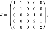
An "almost diagonal" matrix $J$ in Jordan normal form, similar to $A$ is obtained as follows:

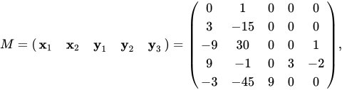
$M={\begin{pmatrix}\mathbf {x} _{1}&\mathbf {x} _{2}&\mathbf {y} _{1}&\mathbf {y} _{2}&\mathbf {y} _{3}\end{pmatrix}}={\begin{pmatrix}0&1&0&0&0\\3&-15&0&0&0\\-9&30&0&0&1\\9&-1&0&3&-2\\-3&-45&9&0&0\end{pmatrix}},$

$J={\begin{pmatrix}1&1&0&0&0\\0&1&0&0&0\\0&0&2&1&0\\0&0&0&2&1\\0&0&0&0&2\end{pmatrix}},$

where $M$ is a generalized modal matrix for $A$ , the columns of $M$ are a canonical basis for $A$ , and $AM=MJ$ .

03Jordan chains

Definition: Let $\mathbf {x} _{m}$ be a generalized eigenvector of rank m corresponding to the matrix $A$ and the eigenvalue $\lambda$ . The chain generated by $\mathbf {x} _{m}$ is a set of vectors $\left\{\mathbf {x} _{m},\mathbf {x} _{m-1},\dots ,\mathbf {x} _{1}\right\}$ given by

$\mathbf {x} _{m-1}=(A-\lambda I)\mathbf {x} _{m},$
$\mathbf {x} _{m-2}=(A-\lambda I)^{2}\mathbf {x} _{m}=(A-\lambda I)\mathbf {x} _{m-1},$
$\mathbf {x} _{m-3}=(A-\lambda I)^{3}\mathbf {x} _{m}=(A-\lambda I)\mathbf {x} _{m-2},$

$\vdots$

$\mathbf {x} _{1}=(A-\lambda I)^{m-1}\mathbf {x} _{m}=(A-\lambda I)\mathbf {x} _{2}.$

where $\mathbf {x} _{1}$ is always an ordinary eigenvector with a given eigenvalue $\lambda$ . Thus, in general,

$\mathbf {x} _{j}=(A-\lambda I)^{m-j}\mathbf {x} _{m}=(A-\lambda I)\mathbf {x} _{j+1}\qquad (j=1,2,\dots ,m-1).$

The vector $\mathbf {x} _{j}$ , given by (2), is a generalized eigenvector of rank j corresponding to the eigenvalue $\lambda$ . A chain is a linearly independent set of vectors.

04Canonical basis

Definition: A set of n linearly independent generalized eigenvectors is a canonical basis if it is composed entirely of Jordan chains.

Thus, once we have determined that a generalized eigenvector of rank m is in a canonical basis, it follows that the m − 1 vectors $\mathbf {x} _{m-1},\mathbf {x} _{m-2},\ldots ,\mathbf {x} _{1}$ that are in the Jordan chain generated by $\mathbf {x} _{m}$ are also in the canonical basis.

Let $\lambda _{i}$ be an eigenvalue of $A$ of algebraic multiplicity $\mu _{i}$ . First, find the ranks (matrix ranks) of the matrices $(A-\lambda _{i}I),(A-\lambda _{i}I)^{2},\ldots ,(A-\lambda _{i}I)^{m_{i}}$ . The integer $m_{i}$ is determined to be the first integer for which $(A-\lambda _{i}I)^{m_{i}}$ has rank $n-\mu _{i}$ (n being the number of rows or columns of $A$ , that is, $A$ is n × n).

Now define

$\rho _{k}=\operatorname {rank} (A-\lambda _{i}I)^{k-1}-\operatorname {rank} (A-\lambda _{i}I)^{k}\qquad (k=1,2,\ldots ,m_{i}).$

The variable $\rho _{k}$ designates the number of linearly independent generalized eigenvectors of rank k corresponding to the eigenvalue $\lambda _{i}$ that will appear in a canonical basis for $A$ . Note that

$\operatorname {rank} (A-\lambda _{i}I)^{0}=\operatorname {rank} (I)=n$ .

05Computation of generalized eigenvectors

In the preceding sections we have seen techniques for obtaining the $n$ linearly independent generalized eigenvectors of a canonical basis for the vector space $V$ associated with an $n\times n$ matrix $A$ . These techniques can be combined into a procedure:

Solve the characteristic equation of $A$ for eigenvalues $\lambda _{i}$ and their algebraic multiplicities $\mu _{i}$ ;

For each $\lambda _{i}:$

Determine $n-\mu _{i}$ ;

Determine $m_{i}$ ;

Determine $\rho _{k}$ for $(k=1,\ldots ,m_{i})$ ;

Determine each Jordan chain for $\lambda _{i}$ ;

Example 3

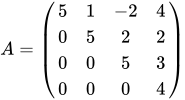
The matrix

$A={\begin{pmatrix}5&1&-2&4\\0&5&2&2\\0&0&5&3\\0&0&0&4\end{pmatrix}}$

has an eigenvalue $\lambda _{1}=5$ of algebraic multiplicity $\mu _{1}=3$ and an eigenvalue $\lambda _{2}=4$ of algebraic multiplicity $\mu _{2}=1$ . We also have $n=4$ . For $\lambda _{1}$ we have $n-\mu _{1}=4-3=1$ .

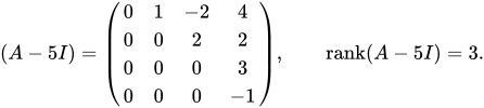
$(A-5I)={\begin{pmatrix}0&1&-2&4\\0&0&2&2\\0&0&0&3\\0&0&0&-1\end{pmatrix}},\qquad \operatorname {rank} (A-5I)=3.$

$(A-5I)^{2}={\begin{pmatrix}0&0&2&-8\\0&0&0&4\\0&0&0&-3\\0&0&0&1\end{pmatrix}},\qquad \operatorname {rank} (A-5I)^{2}=2.$

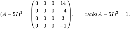
$(A-5I)^{3}={\begin{pmatrix}0&0&0&14\\0&0&0&-4\\0&0&0&3\\0&0&0&-1\end{pmatrix}},\qquad \operatorname {rank} (A-5I)^{3}=1.$

The first integer $m_{1}$ for which $(A-5I)^{m_{1}}$ has rank $n-\mu _{1}=1$ is $m_{1}=3$ .

We now define

$\rho _{3}=\operatorname {rank} (A-5I)^{2}-\operatorname {rank} (A-5I)^{3}=2-1=1,$

$\rho _{2}=\operatorname {rank} (A-5I)^{1}-\operatorname {rank} (A-5I)^{2}=3-2=1,$

$\rho _{1}=\operatorname {rank} (A-5I)^{0}-\operatorname {rank} (A-5I)^{1}=4-3=1.$

Consequently, there will be three linearly independent generalized eigenvectors; one each of ranks 3, 2 and 1. Since $\lambda _{1}$ corresponds to a single chain of three linearly independent generalized eigenvectors, we know that there is a generalized eigenvector $\mathbf {x} _{3}$ of rank 3 corresponding to $\lambda _{1}$ such that

$(A-5I)^{3}\mathbf {x} _{3}=\mathbf {0}$

but

$(A-5I)^{2}\mathbf {x} _{3}\neq \mathbf {0} .$

Equations (3) and (4) represent linear systems that can be solved for $\mathbf {x} _{3}$ . Let

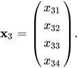
$\mathbf {x} _{3}={\begin{pmatrix}x_{31}\\x_{32}\\x_{33}\\x_{34}\end{pmatrix}}.$

Then

$(A-5I)^{3}\mathbf {x} _{3}={\begin{pmatrix}0&0&0&14\\0&0&0&-4\\0&0&0&3\\0&0&0&-1\end{pmatrix}}{\begin{pmatrix}x_{31}\\x_{32}\\x_{33}\\x_{34}\end{pmatrix}}={\begin{pmatrix}14x_{34}\\-4x_{34}\\3x_{34}\\-x_{34}\end{pmatrix}}={\begin{pmatrix}0\\0\\0\\0\end{pmatrix}}$

and

$(A-5I)^{2}\mathbf {x} _{3}={\begin{pmatrix}0&0&2&-8\\0&0&0&4\\0&0&0&-3\\0&0&0&1\end{pmatrix}}{\begin{pmatrix}x_{31}\\x_{32}\\x_{33}\\x_{34}\end{pmatrix}}={\begin{pmatrix}2x_{33}-8x_{34}\\4x_{34}\\-3x_{34}\\x_{34}\end{pmatrix}}\neq {\begin{pmatrix}0\\0\\0\\0\end{pmatrix}}.$

Thus, in order to satisfy the conditions (3) and (4), we must have $x_{34}=0$ and $x_{33}\neq 0$ . No restrictions are placed on $x_{31}$ and $x_{32}$ . By choosing $x_{31}=x_{32}=x_{34}=0,x_{33}=1$ , we obtain

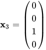
$\mathbf {x} _{3}={\begin{pmatrix}0\\0\\1\\0\end{pmatrix}}$

as a generalized eigenvector of rank 3 corresponding to $\lambda _{1}=5$ . Note that it is possible to obtain infinitely many other generalized eigenvectors of rank 3 by choosing different values of $x_{31}$ , $x_{32}$ and $x_{33}$ , with $x_{33}\neq 0$ . Our first choice, however, is the simplest.

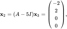
Now using equations (1), we obtain $\mathbf {x} _{2}$ and $\mathbf {x} _{1}$ as generalized eigenvectors of rank 2 and 1, respectively, where

$\mathbf {x} _{2}=(A-5I)\mathbf {x} _{3}={\begin{pmatrix}-2\\2\\0\\0\end{pmatrix}},$

and

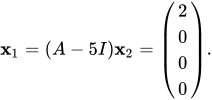
$\mathbf {x} _{1}=(A-5I)\mathbf {x} _{2}={\begin{pmatrix}2\\0\\0\\0\end{pmatrix}}.$

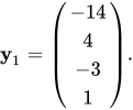
The simple eigenvalue $\lambda _{2}=4$ can be dealt with using standard techniques and has an ordinary eigenvector

$\mathbf {y} _{1}={\begin{pmatrix}-14\\4\\-3\\1\end{pmatrix}}.$

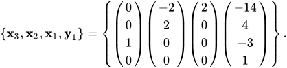
A canonical basis for $A$ is

$\left\{\mathbf {x} _{3},\mathbf {x} _{2},\mathbf {x} _{1},\mathbf {y} _{1}\right\}=\left\{{\begin{pmatrix}0\\0\\1\\0\end{pmatrix}}{\begin{pmatrix}-2\\2\\0\\0\end{pmatrix}}{\begin{pmatrix}2\\0\\0\\0\end{pmatrix}}{\begin{pmatrix}-14\\4\\-3\\1\end{pmatrix}}\right\}.$

$\mathbf {x} _{1},\mathbf {x} _{2}$ and $\mathbf {x} _{3}$ are generalized eigenvectors associated with $\lambda _{1}$ , while $\mathbf {y} _{1}$ is the ordinary eigenvector associated with $\lambda _{2}$ .

This is a fairly simple example. In general, the numbers $\rho _{k}$ of linearly independent generalized eigenvectors of rank $k$ will not always be equal. That is, there may be several chains of different lengths corresponding to a particular eigenvalue.

07Jordan normal form

${\begin{bmatrix}{\color {red}\ulcorner }\lambda _{1}1{\hphantom {\lambda _{1}\lambda _{1}}}{\color {red}\urcorner }{\hphantom {\ulcorner \lambda _{2}1\lambda _{2}\urcorner [\lambda _{3}]\ddots \ulcorner \lambda _{n}1\lambda _{n}\urcorner }}\\{\hphantom {\ulcorner \lambda _{1}1}}\lambda _{1}1{\hphantom {\lambda _{1}\urcorner \ulcorner \lambda _{2}1\lambda _{2}\urcorner [\lambda _{3}]\ddots \ulcorner \lambda _{n}1\lambda _{n}\urcorner }}\\{\color {red}\llcorner }{\hphantom {\lambda _{1}1\lambda _{1}}}\lambda _{1}{\color {red}\lrcorner }{\hphantom {\ulcorner \lambda _{2}1\lambda _{2}\urcorner [\lambda _{3}]\ddots \ulcorner \lambda _{n}1\lambda _{n}\urcorner }}\\{\hphantom {\ulcorner \lambda _{1}1\lambda _{1}1\lambda _{1}\urcorner }}{\color {red}\ulcorner }\lambda _{2}1{\hphantom {n}}{\color {red}\urcorner }{\hphantom {[\lambda _{3}]\ddots \ulcorner \lambda _{n}1\lambda _{n}\urcorner }}\\{\hphantom {\ulcorner \lambda _{1}1\lambda _{1}1\lambda _{1}\lrcorner }}{\color {red}\llcorner }{\hphantom {\lambda _{2}}}\lambda _{2}{\color {red}\lrcorner }{\hphantom {[\lambda _{3}]\ddots \ulcorner \lambda _{n}1\lambda _{n}\urcorner }}\\{\hphantom {\ulcorner \lambda _{1}1\lambda _{1}1\lambda _{1}\urcorner \ulcorner \lambda _{2}1\lambda _{2}\urcorner }}{\color {red}[}\lambda _{3}{\color {red}]}{\hphantom {\ddots \ulcorner \lambda _{n}1\lambda _{n}\urcorner }}\\{\hphantom {\ulcorner \lambda _{1}1\lambda _{1}1\lambda _{1}\urcorner \ulcorner \lambda _{2}1\lambda _{2}\urcorner [\lambda _{3}]}}\ddots {\hphantom {\ulcorner \lambda _{n}1\lambda _{n}\urcorner }}\\{\hphantom {\ulcorner \lambda _{1}1\lambda _{1}1\lambda _{1}\urcorner \ulcorner \lambda _{2}1\lambda _{2}\urcorner [\lambda _{3}]\ddots }}{\color {red}\ulcorner }\lambda _{n}1{\hphantom {n}}{\color {red}\urcorner }\\{\hphantom {\llcorner \lambda _{1}1\lambda _{1}1\lambda _{1}\urcorner \ulcorner \lambda _{2}1\lambda _{2}\urcorner [\lambda _{3}]\ddots }}{\color {red}\llcorner }{\hphantom {\lambda _{n}}}\lambda _{n}{\color {red}\lrcorner }\end{bmatrix}}$ An example of a matrix in Jordan normal form.
The red blocks are called Jordan blocks.

Let $V$ be an n-dimensional vector space; let $\phi$ be a linear map in L(V), the set of all linear maps from $V$ into itself; and let $A$ be the matrix representation of $\phi$ with respect to some ordered basis. It can be shown that if the characteristic polynomial $f(\lambda )$ of $A$ factors into linear factors, so that $f(\lambda )$ has the form

$f(\lambda )=\pm (\lambda -\lambda _{1})^{\mu _{1}}(\lambda -\lambda _{2})^{\mu _{2}}\cdots (\lambda -\lambda _{r})^{\mu _{r}},$

where $\lambda _{1},\lambda _{2},\ldots ,\lambda _{r}$ are the distinct eigenvalues of $A$ , then each $\mu _{i}$ is the algebraic multiplicity of its corresponding eigenvalue $\lambda _{i}$ and $A$ is similar to a matrix $J$ in Jordan normal form, where each $\lambda _{i}$ appears $\mu _{i}$ consecutive times on the diagonal, and the entry directly above each $\lambda _{i}$ (that is, on the superdiagonal) is either 0 or 1: in each block the entry above the first occurrence of each $\lambda _{i}$ is always 0 (except in the first block); all other entries on the superdiagonal are 1. All other entries (that is, off the diagonal and superdiagonal) are 0. (But no ordering is imposed among the eigenvalues, or among the blocks for a given eigenvalue.) The matrix $J$ is as close as one can come to a diagonalization of $A$ . If $A$ is diagonalizable, then all entries above the diagonal are zero. Note that some textbooks have the ones on the subdiagonal, that is, immediately below the main diagonal instead of on the superdiagonal. The eigenvalues are still on the main diagonal.

Every n × n matrix $A$ is similar to a matrix $J$ in Jordan normal form, obtained through the similarity transformation $J=M^{-1}AM$ , where $M$ is a generalized modal matrix for $A$ . (See Note above.)

Example 4

Find a matrix in Jordan normal form that is similar to

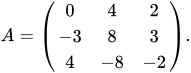
$A={\begin{pmatrix}0&4&2\\-3&8&3\\4&-8&-2\end{pmatrix}}.$

Solution: The characteristic equation of $A$ is $(\lambda -2)^{3}=0$ , hence, $\lambda =2$ is an eigenvalue of algebraic multiplicity three. Following the procedures of the previous sections, we find that

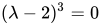
$\operatorname {rank} (A-2I)=1$

and

$\operatorname {rank} (A-2I)^{2}=0=n-\mu .$

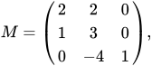
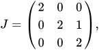
Thus, $\rho _{2}=1$ and $\rho _{1}=2$ , which implies that a canonical basis for $A$ will contain one linearly independent generalized eigenvector of rank 2 and two linearly independent generalized eigenvectors of rank 1, or equivalently, one chain of two vectors $\left\{\mathbf {x} _{2},\mathbf {x} _{1}\right\}$ and one chain of one vector $\left\{\mathbf {y} _{1}\right\}$ . Designating $M={\begin{pmatrix}\mathbf {y} _{1}&\mathbf {x} _{1}&\mathbf {x} _{2}\end{pmatrix}}$ , we find that

$M={\begin{pmatrix}2&2&0\\1&3&0\\0&-4&1\end{pmatrix}},$

and

$J={\begin{pmatrix}2&0&0\\0&2&1\\0&0&2\end{pmatrix}},$

where $M$ is a generalized modal matrix for $A$ , the columns of $M$ are a canonical basis for $A$ , and $AM=MJ$ . Note that since generalized eigenvectors themselves are not unique, and since some of the columns of both $M$ and $J$ may be interchanged, it follows that both $M$ and $J$ are not unique.

Example 5

In Example 3, we found a canonical basis of linearly independent generalized eigenvectors for a matrix $A$ . A generalized modal matrix for $A$ is

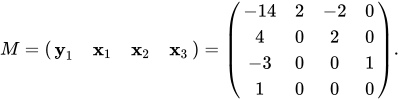
$M={\begin{pmatrix}\mathbf {y} _{1}&\mathbf {x} _{1}&\mathbf {x} _{2}&\mathbf {x} _{3}\end{pmatrix}}={\begin{pmatrix}-14&2&-2&0\\4&0&2&0\\-3&0&0&1\\1&0&0&0\end{pmatrix}}.$

A matrix in Jordan normal form, similar to $A$ is

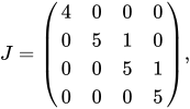
$J={\begin{pmatrix}4&0&0&0\\0&5&1&0\\0&0&5&1\\0&0&0&5\end{pmatrix}},$

so that $AM=MJ$ .

08Applications

Matrix functions

Three of the most fundamental operations which can be performed on square matrices are matrix addition, multiplication by a scalar, and matrix multiplication. These are exactly those operations necessary for defining a polynomial function of an n × n matrix $A$ . If we recall from basic calculus that many functions can be written as a Maclaurin series, then we can define more general functions of matrices quite easily. If $A$ is diagonalizable, that is

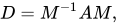
$D=M^{-1}AM,$

with

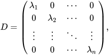
$D={\begin{pmatrix}\lambda _{1}&0&\cdots &0\\0&\lambda _{2}&\cdots &0\\\vdots &\vdots &\ddots &\vdots \\0&0&\cdots &\lambda _{n}\end{pmatrix}},$

then

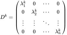
$D^{k}={\begin{pmatrix}\lambda _{1}^{k}&0&\cdots &0\\0&\lambda _{2}^{k}&\cdots &0\\\vdots &\vdots &\ddots &\vdots \\0&0&\cdots &\lambda _{n}^{k}\end{pmatrix}}$

and the evaluation of the Maclaurin series for functions of $A$ is greatly simplified. For example, to obtain any power k of $A$ , we need only compute $D^{k}$ , premultiply $D^{k}$ by $M$ , and postmultiply the result by $M^{-1}$ .

Using generalized eigenvectors, we can obtain the Jordan normal form for $A$ and these results can be generalized to a straightforward method for computing functions of nondiagonalizable matrices. (See Matrix function#Jordan decomposition.)

Differential equations

Consider the problem of solving the system of linear ordinary differential equations

$\mathbf {x} '=A\mathbf {x} ,$

where

$\mathbf {x} ={\begin{pmatrix}x_{1}(t)\\x_{2}(t)\\\vdots \\x_{n}(t)\end{pmatrix}},\quad \mathbf {x} '={\begin{pmatrix}x_{1}'(t)\\x_{2}'(t)\\\vdots \\x_{n}'(t)\end{pmatrix}},$ and $A=(a_{ij}).$

If the matrix $A$ is a diagonal matrix so that $a_{ij}=0$ for $i\neq j$ , then the system (5) reduces to a system of n equations which take the form

$x_{1}'=a_{11}x_{1}$
$x_{2}'=a_{22}x_{2}$

$\vdots$

$x_{n}'=a_{nn}x_{n}.$

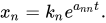
In this case, the general solution is given by

$x_{1}=k_{1}e^{a_{11}t}$

$x_{2}=k_{2}e^{a_{22}t}$

$\vdots$

$x_{n}=k_{n}e^{a_{nn}t}.$

In the general case, we try to diagonalize $A$ and reduce the system (5) to a system like (6) as follows. If $A$ is diagonalizable, we have $D=M^{-1}AM$ , where $M$ is a modal matrix for $A$ . Substituting $A=MDM^{-1}$ , equation (5) takes the form $M^{-1}\mathbf {x} '=D(M^{-1}\mathbf {x} )$ , or

$\mathbf {y} '=D\mathbf {y} ,$

where

$\mathbf {x} =M\mathbf {y} .$

The solution of (7) is

$y_{1}=k_{1}e^{\lambda _{1}t}$

$y_{2}=k_{2}e^{\lambda _{2}t}$

$\vdots$

$y_{n}=k_{n}e^{\lambda _{n}t}.$

The solution $\mathbf {x}$ of (5) is then obtained using the relation (8).

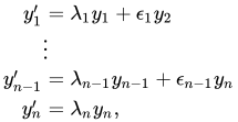
On the other hand, if $A$ is not diagonalizable, we choose $M$ to be a generalized modal matrix for $A$ , such that $J=M^{-1}AM$ is the Jordan normal form of $A$ . The system $\mathbf {y} '=J\mathbf {y}$ has the form

${\begin{aligned}y_{1}'&=\lambda _{1}y_{1}+\epsilon _{1}y_{2}\\&\vdots \\y_{n-1}'&=\lambda _{n-1}y_{n-1}+\epsilon _{n-1}y_{n}\\y_{n}'&=\lambda _{n}y_{n},\end{aligned}}$

where the $\lambda _{i}$ are the eigenvalues from the main diagonal of $J$ and the $\epsilon _{i}$ are the ones and zeros from the superdiagonal of $J$ . The system (9) is often more easily solved than (5). We may solve the last equation in (9) for $y_{n}$ , obtaining $y_{n}=k_{n}e^{\lambda _{n}t}$ . We then substitute this solution for $y_{n}$ into the next to last equation in (9) and solve for $y_{n-1}$ . Continuing this procedure, we work through (9) from the last equation to the first, solving the entire system for $\mathbf {y}$ . The solution $\mathbf {x}$ is then obtained using the relation (8).

Lemma:

Given the following chain of generalized eigenvectors of length $r,$

$X_{1}=v_{1}e^{\lambda t}$

$X_{2}=(tv_{1}+v_{2})e^{\lambda t}$

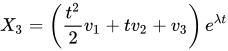
$X_{3}=\left({\frac {t^{2}}{2}}v_{1}+tv_{2}+v_{3}\right)e^{\lambda t}$

$\vdots$

$X_{r}=\left({\frac {t^{r-1}}{(r-1)!}}v_{1}+...+{\frac {t^{2}}{2}}v_{r-2}+tv_{r-1}+v_{r}\right)e^{\lambda t}$ ,

these functions solve the system of equations,

$X'=AX.$

Proof:

Define

$v_{0}=0$

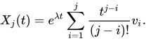
$X_{j}(t)=e^{\lambda t}\sum _{i=1}^{j}{\frac {t^{j-i}}{(j-i)!}}v_{i}.$

Then, as ${t^{0}}=1$ and $1'=0$ ,

$X'_{j}(t)=e^{\lambda t}\sum _{i=1}^{j-1}{\frac {t^{j-i-1}}{(j-i-1)!}}v_{i}+e^{\lambda t}\lambda \sum _{i=1}^{j}{\frac {t^{j-i}}{(j-i)!}}v_{i}$ .

On the other hand we have, $v_{0}=0$ and so

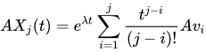
$AX_{j}(t)=e^{\lambda t}\sum _{i=1}^{j}{\frac {t^{j-i}}{(j-i)!}}Av_{i}$

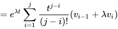
$=e^{\lambda t}\sum _{i=1}^{j}{\frac {t^{j-i}}{(j-i)!}}(v_{i-1}+\lambda v_{i})$

$=e^{\lambda t}\sum _{i=2}^{j}{\frac {t^{j-i}}{(j-i)!}}v_{i-1}+e^{\lambda t}\lambda \sum _{i=1}^{j}{\frac {t^{j-i}}{(j-i)!}}v_{i}$

$=e^{\lambda t}\sum _{i=1}^{j-1}{\frac {t^{j-i-1}}{(j-i-1)!}}v_{i}+e^{\lambda t}\lambda \sum _{i=1}^{j}{\frac {t^{j-i}}{(j-i)!}}v_{i}$

$=X'_{j}(t)$

as required.

Watch videos about Generalized eigenvectorExplainers and documentaries on YouTube (opens in a new tab)

Sources and credits

This article is adapted from the Wikipedia article “Generalized eigenvector”, written by its contributors and licensed under CC BY-SA 4.0. Fathomly has changed the layout, removed citation markers, navigation and maintenance notices, and adjusted punctuation. This adapted version is shared under the same license. For references, see the original article.

Fathomly is not affiliated with or endorsed by the Wikimedia Foundation. Spotted a problem? Tell us.

Generalized eigenvector

01Overview and definition

02Examples

Example 1

Example 2

03Jordan chains

04Canonical basis

05Computation of generalized eigenvectors

Example 3

06Generalized modal matrix

07Jordan normal form

Example 4

Example 5

08Applications

Matrix functions

Differential equations

Sources and credits