Encyclopedia

Autoregressive conditional heteroskedasticity

Time series model

Wikipedia contributorsAdapted for Fathomly · View authors

7 min read
Source updated August 29, 2026

In econometrics, the autoregressive conditional heteroskedasticity (ARCH) model is a statistical model for time series data that describes the variance of the current error term or innovation as a function of the actual sizes of the previous time periods' error terms; often the variance is related to the squares of the previous innovations. The ARCH model is appropriate when the error variance in a time series follows an autoregressive (AR) model; if an autoregressive moving average (ARMA) model is assumed for the error variance, the model is a generalized autoregressive conditional heteroskedasticity (GARCH) model.

ARCH models are commonly employed in modeling financial time series that exhibit time-varying volatility and volatility clustering, i.e. periods of swings interspersed with periods of relative calm (this is, when the time series exhibits heteroskedasticity). ARCH-type models are sometimes considered to be in the family of stochastic volatility models, although this is strictly incorrect since at time t the volatility is completely predetermined (deterministic) given previous values.

01Model specification

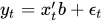
To model a time series using an ARCH process, let $~\epsilon _{t}~$ denote the error terms (return residuals, with respect to a mean process), i.e. the series terms. These $~\epsilon _{t}~$ are split into a stochastic piece $z_{t}$ and a time-dependent standard deviation $\sigma _{t}$ characterizing the typical size of the terms so that

$~\epsilon _{t}=\sigma _{t}z_{t}~$

The random variable $z_{t}$ is a strong white noise process. The series $\sigma _{t}^{2}$ is modeled by

$\sigma _{t}^{2}=\alpha _{0}+\alpha _{1}\epsilon _{t-1}^{2}+\cdots +\alpha _{q}\epsilon _{t-q}^{2}=\alpha _{0}+\sum _{i=1}^{q}\alpha _{i}\epsilon _{t-i}^{2}$ ,

where $~\alpha _{0}>0~$ and $\alpha _{i}\geq 0,~i>0$ .

An ARCH(q) model can be estimated using ordinary least squares. A method for testing whether the residuals $\epsilon _{t}$ exhibit time-varying heteroskedasticity using the Lagrange multiplier test was proposed by Engle (1982). This procedure is as follows:

Estimate the best fitting autoregressive model AR(q) $y_{t}=a_{0}+a_{1}y_{t-1}+\cdots +a_{q}y_{t-q}+\epsilon _{t}=a_{0}+\sum _{i=1}^{q}a_{i}y_{t-i}+\epsilon _{t}$ .
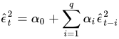
Obtain the squares of the error ${\hat {\epsilon }}^{2}$ and regress them on a constant and q lagged values:
${\hat {\epsilon }}_{t}^{2}=\alpha _{0}+\sum _{i=1}^{q}\alpha _{i}{\hat {\epsilon }}_{t-i}^{2}$

where q is the length of ARCH lags.
The null hypothesis is that, in the absence of ARCH components, we have $\alpha _{i}=0$ for all $i=1,\cdots ,q$ . The alternative hypothesis is that, in the presence of ARCH components, at least one of the estimated $\alpha _{i}$ coefficients must be significant. In a sample of T residuals under the null hypothesis of no ARCH errors, the test statistic T'R² follows $\chi ^{2}$ distribution with q degrees of freedom, where $T'$ is the number of equations in the model which fits the residuals vs the lags (i.e. $T'=T-q$ ). If T'R² is greater than the Chi-square table value, we reject the null hypothesis and conclude there is an ARCH effect in the ARMA model. If T'R² is smaller than the Chi-square table value, we do not reject the null hypothesis.

02GARCH

If an autoregressive moving average (ARMA) model is assumed for the error variance, the model is a generalized autoregressive conditional heteroskedasticity (GARCH) model.

In that case, the GARCH (p, q) model (where p is the order of the GARCH terms $~\sigma ^{2}$ and q is the order of the ARCH terms $~\epsilon ^{2}$ ), following the notation of the original paper, is given by

$y_{t}=x'_{t}b+\epsilon _{t}$

$\epsilon _{t}|y_{t-1}\sim {\mathcal {N}}(0,\sigma _{t}^{2})$

$\sigma _{t}^{2}=\omega +\alpha _{1}\epsilon _{t-1}^{2}+\cdots +\alpha _{q}\epsilon _{t-q}^{2}+\beta _{1}\sigma _{t-1}^{2}+\cdots +\beta _{p}\sigma _{t-p}^{2}=\omega +\sum _{i=1}^{q}\alpha _{i}\epsilon _{t-i}^{2}+\sum _{i=1}^{p}\beta _{i}\sigma _{t-i}^{2}$

Generally, when testing for heteroskedasticity in econometric models, the best test is the White test. However, when dealing with time series data, this means to test for ARCH and GARCH errors.

Exponentially weighted moving average (EWMA) is an alternative model in a separate class of exponential smoothing models. As an alternative to GARCH modelling it has some attractive properties such as a greater weight upon more recent observations, but also drawbacks such as an arbitrary decay factor that introduces subjectivity into the estimation.

GARCH(p, q) model specification

The lag length p of a GARCH(p, q) process is established in three steps:

Estimate the best fitting AR(q) model
$y_{t}=a_{0}+a_{1}y_{t-1}+\cdots +a_{q}y_{t-q}+\epsilon _{t}=a_{0}+\sum _{i=1}^{q}a_{i}y_{t-i}+\epsilon _{t}$ .
Compute and plot the autocorrelations of $\epsilon ^{2}$ by
$\rho (i)={{\sum _{t=i+1}^{T}({\hat {\epsilon }}_{t}^{2}-{\hat {\sigma }}_{t}^{2})({\hat {\epsilon }}_{t-i}^{2}-{\hat {\sigma }}_{t-i}^{2})} \over {\sum _{t=1}^{T}({\hat {\epsilon }}_{t}^{2}-{\hat {\sigma }}_{t}^{2})^{2}}}$
The asymptotic, that is for large samples, standard deviation of $\rho (i)$ is $1/{\sqrt {T}}$ . Individual values that are larger than this indicate GARCH errors. To estimate the total number of lags, use the Ljung-Box test until the value of these are less than, say, 10% significant. The Ljung-Box Q-statistic follows $\chi ^{2}$ distribution with n degrees of freedom if the squared residuals $\epsilon _{t}^{2}$ are uncorrelated. It is recommended to consider up to T/4 values of n. The null hypothesis states that there are no ARCH or GARCH errors. Rejecting the null thus means that such errors exist in the conditional variance.

NGARCH

NAGARCH

Nonlinear Asymmetric GARCH(1,1) (NAGARCH) is a model with the specification:

$~\sigma _{t}^{2}=~\omega +~\alpha (~\epsilon _{t-1}-~\theta ~\sigma _{t-1})^{2}+~\beta ~\sigma _{t-1}^{2}$ ,

where $~\alpha \geq 0,~\beta \geq 0,~\omega >0$ and $~\alpha (1+~\theta ^{2})+~\beta <1$ , which ensures the non-negativity and stationarity of the variance process.

For stock returns, parameter $~\theta$ is usually estimated to be positive; in this case, it reflects a phenomenon commonly referred to as the "leverage effect", signifying that negative returns increase future volatility by a larger amount than positive returns of the same magnitude.

This model should not be confused with the NARCH model, together with the NGARCH extension, introduced by Higgins and Bera in 1992.

IGARCH

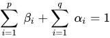
Integrated Generalized Autoregressive Conditional heteroskedasticity (IGARCH) is a restricted version of the GARCH model, where the persistent parameters sum up to one, and imports a unit root in the GARCH process. The condition for this is

$\sum _{i=1}^{p}~\beta _{i}+\sum _{i=1}^{q}~\alpha _{i}=1$ .

EGARCH

The exponential generalized autoregressive conditional heteroskedastic (EGARCH) model by Nelson & Cao (1991) is another form of the GARCH model. Formally, an EGARCH(p,q):

$\log \sigma _{t}^{2}=\omega +\sum _{k=1}^{q}\beta _{k}g(Z_{t-k})+\sum _{k=1}^{p}\alpha _{k}\log \sigma _{t-k}^{2}$

where $g(Z_{t})=\theta Z_{t}+\lambda (|Z_{t}|-E(|Z_{t}|))$ , $\sigma _{t}^{2}$ is the conditional variance, $\omega$ , $\beta$ , $\alpha$ , $\theta$ and $\lambda$ are coefficients. $Z_{t}$ may be a standard normal variable or come from a generalized error distribution. The formulation for $g(Z_{t})$ allows the sign and the magnitude of $Z_{t}$ to have separate effects on the volatility. This is particularly useful in an asset pricing context.

Since $\log \sigma _{t}^{2}$ may be negative, there are no sign restrictions for the parameters.

GARCH-M

The GARCH-in-mean (GARCH-M) model adds a heteroskedasticity term into the mean equation. It has the specification:

$y_{t}=~\beta x_{t}+~\lambda ~\sigma _{t}+~\epsilon _{t}$

The residual $~\epsilon _{t}$ is defined as:

$~\epsilon _{t}=~\sigma _{t}~\times z_{t}$

QGARCH

The Quadratic GARCH (QGARCH) model by Sentana (1995) is used to model asymmetric effects of positive and negative shocks.

In the example of a GARCH(1,1) model, the residual process $~\sigma _{t}$ is

$~\epsilon _{t}=~\sigma _{t}z_{t}$

where $z_{t}$ is i.i.d. and

$~\sigma _{t}^{2}=K+~\alpha ~\epsilon _{t-1}^{2}+~\beta ~\sigma _{t-1}^{2}+~\phi ~\epsilon _{t-1}$

GJR-GARCH

Similar to QGARCH, the Glosten-Jagannathan-Runkle GARCH (GJR-GARCH) model by Glosten, Jagannathan and Runkle (1993) also models asymmetry in the ARCH process. The suggestion is to model $~\epsilon _{t}=~\sigma _{t}z_{t}$ where $z_{t}$ is i.i.d., and

$~\sigma _{t}^{2}=K+~\delta ~\sigma _{t-1}^{2}+~\alpha ~\epsilon _{t-1}^{2}+~\phi ~\epsilon _{t-1}^{2}I_{t-1}$

where $I_{t-1}=0$ if $~\epsilon _{t-1}\geq 0$ , and $I_{t-1}=1$ if $~\epsilon _{t-1}<0$ .

TGARCH model

The Threshold GARCH (TGARCH) model by Zakoian (1994) is similar to GJR GARCH. The specification is one on conditional standard deviation instead of conditional variance:

$~\sigma _{t}=K+~\delta ~\sigma _{t-1}+~\alpha _{1}^{+}~\epsilon _{t-1}^{+}+~\alpha _{1}^{-}~\epsilon _{t-1}^{-}$

where $~\epsilon _{t-1}^{+}=~\epsilon _{t-1}$ if $~\epsilon _{t-1}>0$ , and $~\epsilon _{t-1}^{+}=0$ if $~\epsilon _{t-1}\leq 0$ . Likewise, $~\epsilon _{t-1}^{-}=~\epsilon _{t-1}$ if $~\epsilon _{t-1}\leq 0$ , and $~\epsilon _{t-1}^{-}=0$ if $~\epsilon _{t-1}>0$ .

fGARCH

Hentschel's fGARCH model, also known as Family GARCH, is an omnibus model that nests a variety of other popular symmetric and asymmetric GARCH models including APARCH, GJR, AVGARCH, NGARCH, etc.

COGARCH

In 2004, Claudia Klüppelberg, Alexander Lindner and Ross Maller proposed a continuous-time generalization of the discrete-time GARCH(1,1) process. The idea is to start with the GARCH(1,1) model equations

$\epsilon _{t}=\sigma _{t}z_{t},$

$\sigma _{t}^{2}=\alpha _{0}+\alpha _{1}\epsilon _{t-1}^{2}+\beta _{1}\sigma _{t-1}^{2}=\alpha _{0}+\alpha _{1}\sigma _{t-1}^{2}z_{t-1}^{2}+\beta _{1}\sigma _{t-1}^{2},$

and then to replace the strong white noise process $z_{t}$ by the infinitesimal increments $\mathrm {d} L_{t}$ of a Lévy process $(L_{t})_{t\geq 0}$ , and the squared noise process $z_{t}^{2}$ by the increments $\mathrm {d} [L,L]_{t}^{\mathrm {d} }$ , where

$[L,L]_{t}^{\mathrm {d} }=\sum _{s\in [0,t]}(\Delta L_{t})^{2},\quad t\geq 0,$

is the purely discontinuous part of the quadratic variation process of $L$ . The result is the following system of stochastic differential equations:

$\mathrm {d} G_{t}=\sigma _{t-}\,\mathrm {d} L_{t},$

$\mathrm {d} \sigma _{t}^{2}=(\beta -\eta \sigma _{t}^{2})\,\mathrm {d} t+\varphi \sigma _{t-}^{2}\,\mathrm {d} [L,L]_{t}^{\mathrm {d} },$

where the positive parameters $\beta$ , $\eta$ and $\varphi$ are determined by $\alpha _{0}$ , $\alpha _{1}$ and $\beta _{1}$ . Now given some initial condition $(G_{0},\sigma _{0}^{2})$ , the system above has a pathwise unique solution $(G_{t},\sigma _{t}^{2})_{t\geq 0}$ which is then called the continuous-time GARCH (COGARCH) model.

MF2-GARCH

The multiplicative factor multi-frequency GARCH (MF2-GARCH) was proposed by Conrad and Engle (2025), and it features stationary returns and allows for recursive long-term volatility forecasts. They exploit the fact that daily standardized volatility forecast errors of one-component GARCH models are essentially unpredictable based on past daily standardized forecast errors, but a rolling window moving average of past daily standardized forecast errors does have predictive power. The MF2-GARCH, $\epsilon _{t}={\sqrt {\sigma _{t}^{2}\tau _{t}}}z_{t}$ , where $z_{t}$ is standard Gaussian, combines a short-term GJR-GARCH component

$h_{t}=(1-\phi )+\left(\alpha +\gamma \mathbf {1} _{\{\eta _{d,t-1}<0\}}\right){\frac {\eta _{d,t-1}^{2}}{\tau _{t-1}}}+\beta h_{t-1}$

with $~\alpha >0,\alpha +\gamma >0,\beta >0$ and $~\phi =\alpha +\gamma /2+\beta <1$ , and a long-term component specified as a multiplicative error model (MEM) for the past forecast errors of the GARCH component, exploiting the predictability in the averaged standardized forecast errors of the short-term component.

$\tau _{t}=\lambda _{0}+\lambda _{1}{\frac {1}{m}}\sum _{j=1}^{m}{\frac {\eta _{d,t-j}^{2}}{h_{t-j}}}+\lambda _{2}\tau _{t-1}$

with $~\lambda _{0}>0,\lambda _{1}>0,\lambda _{2}>0$ and $~\lambda _{1}+\lambda _{2}<1$ . $m$ is chosen by minimizing the Bayesian Information Criterion (BIC, SIC).

Empirically, the long-term volatility component is closely linked to news about macroeconomics and monetary policy. The immediate reaction of stock market indices to U.S. macroeconomic announcements (e.g., initial jobless claims or incoming orders) depends on the level of long-term stock market volatility.

ZD-GARCH

An ARCH model without intercept was proposed by Hafner and Preminger (2015), who set the intercept term to zero ( $~\omega =0$ ), in the first order ARCH model $~\epsilon _{t}=~\sigma _{t}z_{t}$ , where $z_{t}$ is i.i.d., and the conditional variance is:

$~\sigma _{t}^{2}=~\alpha _{1}~\epsilon _{t-1}^{2}.$

This model was extended by Li, Zhang, Zhu and Ling (2018) which consider the Zero-Drift GARCH (ZD-GARCH) with the specification:

$~\sigma _{t}^{2}=~\alpha _{1}~\epsilon _{t-1}^{2}+~\beta _{1}~\sigma _{t-1}^{2}.$

The ZD-GARCH model does not require $~\alpha _{1}+~\beta _{1}=1$ , and hence it nests the Exponentially weighted moving average (EWMA) model in "RiskMetrics". Since $~\omega =0$ , the ZD-GARCH model is always non-stationary, and its statistical inference methods are quite different from those for the classical GARCH model. Based on the historical data, the parameters $~\alpha _{1}$ and $~\beta _{1}$ can be estimated by the generalized QMLE method.

Spatial and Spatiotemporal GARCH

Spatial GARCH processes by Otto, Schmid and Garthoff (2018) are considered as the spatial equivalent to the temporal generalized autoregressive conditional heteroscedasticity (GARCH) models. In contrast to the temporal ARCH model, in which the distribution is known given the full information set for the prior periods, the distribution is not straightforward in the spatial and spatiotemporal setting due to the contemporaneous dependence between neighboring spatial locations. The spatial model is given by $~\epsilon (s_{i})=~\sigma (s_{i})z(s_{i})$ and

$~\sigma (s_{i})^{2}=~\alpha _{i}+\sum _{v=1}^{n}\rho w_{iv}\epsilon (s_{v})^{2},$

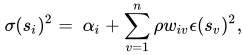
where $~s_{i}$ denotes the $i$ -th spatial location and $~w_{iv}$ refers to the $iv$ -th entry of a spatial weight matrix and $w_{ii}=0$ for $~i=1,...,n$ . The spatial weight matrix defines which locations are considered to be adjacent.

In spatiotemporal extensions, the conditional variance is modelled as a joint function of spatially lagged past squared observations and temporally lagged volatilities, allowing for both cross-sectional and serial dependence. These models have been applied in fields such as environmental statistics, regional economics, and financial econometrics, where shocks can propagate over space and time. Recent reviews summarise methodological developments, estimation techniques, and applications across disciplines.

03Gaussian process-driven GARCH

In a different vein, the machine learning community has proposed the use of Gaussian process regression models to obtain a GARCH scheme. This results in a nonparametric modelling scheme, which allows for: (i) advanced robustness to overfitting, since the model marginalises over its parameters to perform inference, under a Bayesian inference rationale; and (ii) capturing highly-nonlinear dependencies without increasing model complexity.

Watch videos about Autoregressive conditional heteroskedasticityExplainers and documentaries on YouTube (opens in a new tab)

Sources and credits

This article is adapted from the Wikipedia article “Autoregressive conditional heteroskedasticity”, written by its contributors and licensed under CC BY-SA 4.0. Fathomly has changed the layout, removed citation markers, navigation and maintenance notices, and adjusted punctuation. This adapted version is shared under the same license. For references, see the original article.

Fathomly is not affiliated with or endorsed by the Wikimedia Foundation. Spotted a problem? Tell us.