Encyclopedia

Conditional probability distribution

Probability theory and statistics concept

Wikipedia contributorsAdapted for Fathomly · View authors

5 min read
Source updated January 26, 2026

In probability theory and statistics, the conditional probability distribution is a probability distribution that describes the probability of an outcome given the occurrence of a particular event. Given two jointly distributed random variables $X$ and $Y$ , the conditional probability distribution of $Y$ given $X$ is the probability distribution of $Y$ when $X$ is known to be a particular value; in some cases the conditional probabilities may be expressed as functions containing the unspecified value $x$ of $X$ as a parameter. When both $X$ and $Y$ are categorical variables, a conditional probability table is typically used to represent the conditional probability. The conditional distribution contrasts with the marginal distribution of a random variable, which is its distribution without reference to the value of the other variable.

If the conditional distribution of $Y$ given $X$ is a continuous distribution, then its probability density function is known as the conditional density function. The properties of a conditional distribution, such as the moments, are often referred to by corresponding names such as the conditional mean and conditional variance.

More generally, one can refer to the conditional distribution of a subset of a set of more than two variables; this conditional distribution is contingent on the values of all the remaining variables, and if more than one variable is included in the subset then this conditional distribution is the conditional joint distribution of the included variables.

01Conditional discrete distributions

For discrete random variables, the conditional probability mass function of $Y$ given $X=x$ can be written according to its definition as:

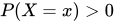
$p_{Y|X}(y\mid x)\triangleq P(Y=y\mid X=x)={\frac {P(\{X=x\}\cap \{Y=y\})}{P(X=x)}}\qquad$

Due to the occurrence of $P(X=x)$ in the denominator, this is defined only for non-zero (hence strictly positive) $P(X=x).$

The relation with the probability distribution of $X$ given $Y$ is:

$P(Y=y\mid X=x)P(X=x)=P(\{X=x\}\cap \{Y=y\})=P(X=x\mid Y=y)P(Y=y).$

Example

Consider the roll of a fair die and let $X=1$ if the number is even (i.e., 2, 4, or 6) and $X=0$ otherwise. Furthermore, let $Y=1$ if the number is prime (i.e., 2, 3, or 5) and $Y=0$ otherwise.

D	1	2	3	4	5	6
X	0	1	0	1	0	1
Y	0	1	1	0	1	0

Then the unconditional probability that $X=1$ is 3/6 = 1/2 (since there are six possible rolls of the die, of which three are even), whereas the probability that $X=1$ conditional on $Y=1$ is 1/3 (since there are three possible prime number rolls, 2, 3, and 5, of which one is even).

02Conditional continuous distributions

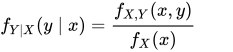
Similarly for continuous random variables, the conditional probability density function of $Y$ given the occurrence of the value $x$ of $X$ can be written as

$f_{Y\mid X}(y\mid x)={\frac {f_{X,Y}(x,y)}{f_{X}(x)}}\qquad$

where $f_{X,Y}(x,y)$ gives the joint density of $X$ and $Y$ , while $f_{X}(x)$ gives the marginal density for $X$ . Also in this case it is necessary that $f_{X}(x)>0$ .

The relation with the probability distribution of $X$ given $Y$ is given by:

$f_{Y\mid X}(y\mid x)f_{X}(x)=f_{X,Y}(x,y)=f_{X|Y}(x\mid y)f_{Y}(y).$

The concept of the conditional distribution of a continuous random variable is not as intuitive as it might seem: Borel's paradox shows that conditional probability density functions need not be invariant under coordinate transformations.

Example

The graph shows a bivariate normal joint density for random variables $X$ and $Y$ . To see the distribution of $Y$ conditional on $X=70$ , one can first visualize the line $X=70$ in the $X,Y$ plane, and then visualize the plane containing that line and perpendicular to the $X,Y$ plane. The intersection of that plane with the joint normal density, once rescaled to give unit area under the intersection, is the relevant conditional density of $Y$ .

$Y\mid X=70\ \sim \ {\mathcal {N}}\left(\mu _{Y}+{\frac {\sigma _{Y}}{\sigma _{X}}}\rho (70-\mu _{X}),\,(1-\rho ^{2})\sigma _{Y}^{2}\right).$

03Relation to independence

Random variables $X$ , $Y$ are independent if and only if the conditional distribution of $Y$ given $X$ is, for all possible realizations of $X$ , equal to the unconditional distribution of $Y$ . For discrete random variables this means $P(Y=y|X=x)=P(Y=y)$ for all possible $y$ and $x$ with $P(X=x)>0$ . For continuous random variables $X$ and $Y$ , having a joint density function, it means $f_{Y}(y|X=x)=f_{Y}(y)$ for all possible $y$ and $x$ with $f_{X}(x)>0$ .

04Properties

Seen as a function of $y$ for given $x$ , $P(Y=y|X=x)$ is a probability mass function and so the sum over all $y$ (or integral if it is a conditional probability density) is 1. Seen as a function of $x$ for given $y$ , it is a likelihood function, so that the sum (or integral) over all $x$ need not be 1.

Additionally, a marginal of a joint distribution can be expressed as the expectation of the corresponding conditional distribution. For instance, $p_{X}(x)=E_{Y}[p_{X|Y}(x\ |\ Y)]$ .

05Measure-theoretic formulation

Let $(\Omega ,{\mathcal {F}},P)$ be a probability space, ${\mathcal {G}}\subseteq {\mathcal {F}}$ a $\sigma$ -field in ${\mathcal {F}}$ . Given $A\in {\mathcal {F}}$ , the Radon-Nikodym theorem implies that there is a ${\mathcal {G}}$ -measurable random variable $P(A\mid {\mathcal {G}}):\Omega \to \mathbb {R}$ , called the conditional probability, such that $\int _{G}P(A\mid {\mathcal {G}})(\omega )dP(\omega )=P(A\cap G)$ for every $G\in {\mathcal {G}}$ , and such a random variable is uniquely defined up to sets of probability zero. A conditional probability is called regular if $\operatorname {P} (\cdot \mid {\mathcal {G}})(\omega )$ is a probability measure on $(\Omega ,{\mathcal {F}})$ for all $\omega \in \Omega$ a.e.

Special cases:

For the trivial sigma algebra ${\mathcal {G}}=\{\emptyset ,\Omega \}$ , the conditional probability is the constant function $\operatorname {P} \!\left(A\mid \{\emptyset ,\Omega \}\right)=\operatorname {P} (A).$
If $A\in {\mathcal {G}}$ , then $\operatorname {P} (A\mid {\mathcal {G}})=1_{A}$ , the indicator function (defined below).

Let $X:\Omega \to E$ be a $(E,{\mathcal {E}})$ -valued random variable. For each $B\in {\mathcal {E}}$ , define $\mu _{X\,|\,{\mathcal {G}}}(B\,|\,{\mathcal {G}})=\mathrm {P} (X^{-1}(B)\,|\,{\mathcal {G}}).$ For any $\omega \in \Omega$ , the function $\mu _{X\,|{\mathcal {G}}}(\cdot \,|{\mathcal {G}})(\omega ):{\mathcal {E}}\to \mathbb {R}$ is called the conditional probability distribution of $X$ given ${\mathcal {G}}$ . If it is a probability measure on $(E,{\mathcal {E}})$ , then it is called regular.

For a real-valued random variable (with respect to the Borel $\sigma$ -field ${\mathcal {R}}^{1}$ on $\mathbb {R}$ ), every conditional probability distribution is regular. In this case, $E[X\mid {\mathcal {G}}]=\int _{-\infty }^{\infty }x\,\mu _{X\mid {\mathcal {G}}}(dx,\cdot )$ almost surely.

Relation to conditional expectation

For any event $A\in {\mathcal {F}}$ , define the indicator function:

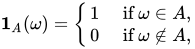
$\mathbf {1} _{A}(\omega )={\begin{cases}1\;&{\text{if }}\omega \in A,\\0\;&{\text{if }}\omega \notin A,\end{cases}}$

which is a random variable. Note that the expectation of this random variable is equal to the probability of A itself:

$\operatorname {E} (\mathbf {1} _{A})=\operatorname {P} (A).\;$

Given a $\sigma$ -field ${\mathcal {G}}\subseteq {\mathcal {F}}$ , the conditional probability $\operatorname {P} (A\mid {\mathcal {G}})$ is a version of the conditional expectation of the indicator function for $A$ :

$\operatorname {P} (A\mid {\mathcal {G}})=\operatorname {E} (\mathbf {1} _{A}\mid {\mathcal {G}})\;$

An expectation of a random variable with respect to a regular conditional probability is equal to its conditional expectation.

Interpretation of conditioning on a Sigma Field

Consider the probability space $(\Omega ,{\mathcal {F}},\mathbb {P} )$ and a sub-sigma field ${\mathcal {A}}\subset {\mathcal {F}}$ . The sub-sigma field ${\mathcal {A}}$ can be loosely interpreted as containing a subset of the information in ${\mathcal {F}}$ . For example, we might think of $\mathbb {P} (B|{\mathcal {A}})$ as the probability of the event $B$ given the information in ${\mathcal {A}}$ .

Also recall that an event $B$ is independent of a sub-sigma field ${\mathcal {A}}$ if $\mathbb {P} (B|A)=\mathbb {P} (B)$ for all $A\in {\mathcal {A}}$ . It is incorrect to conclude in general that the information in ${\mathcal {A}}$ does not tell us anything about the probability of event $B$ occurring. This can be shown with a counter-example:

Consider a probability space on the unit interval, $\Omega =[0,1]$ . Let ${\mathcal {G}}$ be the sigma-field of all countable sets and sets whose complement is countable. So each set in ${\mathcal {G}}$ has measure $0$ or $1$ and so is independent of each event in ${\mathcal {F}}$ . However, notice that ${\mathcal {G}}$ also contains all the singleton events in ${\mathcal {F}}$ (those sets which contain only a single $\omega \in \Omega$ ). So knowing which of the events in ${\mathcal {G}}$ occurred is equivalent to knowing exactly which $\omega \in \Omega$ occurred! So in one sense, ${\mathcal {G}}$ contains no information about ${\mathcal {F}}$ (it is independent of it), and in another sense it contains all the information in ${\mathcal {F}}$ .

Watch videos about Conditional probability distributionExplainers and documentaries on YouTube (opens in a new tab)

Sources and credits

This article is adapted from the Wikipedia article “Conditional probability distribution”, written by its contributors and licensed under CC BY-SA 4.0. Fathomly has changed the layout, removed citation markers, navigation and maintenance notices, and adjusted punctuation. This adapted version is shared under the same license. For references, see the original article.

Images, from Wikimedia Commons:

Multivariate Gaussian.png by Unknown author, CC BY-SA 3.0

Fathomly is not affiliated with or endorsed by the Wikimedia Foundation. Spotted a problem? Tell us.

Conditional probability distribution

01Conditional discrete distributions

Example

02Conditional continuous distributions

Example

03Relation to independence

04Properties

05Measure-theoretic formulation

Relation to conditional expectation

Interpretation of conditioning on a Sigma Field

Sources and credits

Related topics

Conditioning (probability)

Conditional probability

Regular conditional probability