Encyclopedia

Conditional expectation

Expected value of a random variable given that certain conditions are known to occur

Wikipedia contributorsAdapted for Fathomly · View authors

10 min read
Source updated July 13, 2026

In probability theory, the conditional expectation, conditional expected value, or conditional mean of a random variable is its expected value evaluated with respect to the conditional probability distribution. If the random variable can take on only a finite number of values, the "conditions" are that the variable can only take on a subset of those values. More formally, in the case when the random variable is defined over a discrete probability space, the "conditions" are a partition of this probability space.

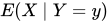
Depending on the context, the conditional expectation can be either a random variable or a function. The random variable is denoted $E(X\mid Y)$ analogously to conditional probability. The function form is either denoted $E(X\mid Y=y)$ or a separate function symbol such as $f(y)$ is introduced with the meaning $E(X\mid Y)=f(Y)$ .

01Examples

Example 1: Dice rolling

Consider the roll of a fair dice and let A = 1 if the number is even (i.e., 2, 4, or 6) and A = 0 otherwise. Furthermore, let B = 1 if the number is prime (i.e., 2, 3, or 5) and B = 0 otherwise.

	1	2	3	4	5	6
A	0	1	0	1	0	1
B	0	1	1	0	1	0

The unconditional expectation of A is $E[A]=(0+1+0+1+0+1)/6=1/2$ , but the expectation of A conditional on B = 1 (i.e., conditional on the die roll being 2, 3, or 5) is $E[A\mid B=1]=(1+0+0)/3=1/3$ , and the expectation of A conditional on B = 0 (i.e., conditional on the die roll being 1, 4, or 6) is $E[A\mid B=0]=(0+1+1)/3=2/3$ . Likewise, the expectation of B conditional on A = 1 is $E[B\mid A=1]=(1+0+0)/3=1/3$ , and the expectation of B conditional on A = 0 is $E[B\mid A=0]=(0+1+1)/3=2/3$ .

Example 2: Rainfall data

Suppose we have daily rainfall data (mm of rain each day) collected by a weather station on every day of the ten-year (3652-day) period from January 1, 1990, to December 31, 1999. The unconditional expectation of rainfall for an unspecified day is the average of the rainfall amounts for those 3652 days. The conditional expectation of rainfall for an otherwise unspecified day known to be (conditional on being) in the month of March, is the average of daily rainfall over all 310 days of the ten-year period that fall in March. Similarly, the conditional expectation of rainfall conditional on days dated March 2 is the average of the rainfall amounts that occurred on the ten days with that specific date.

Conditional expectation with respect to a σ-algebra: in this example the probability space is the [0,1] interval with the Lebesgue measure. We define the following σ-algebras: ; is the σ-algebra generated by the intervals with end-points 0, 1⁄4, 1⁄2, 3⁄4, 1; and is the σ-algebra generated by the intervals with end-points 0, 1⁄2, 1. Here the conditional expectation is effectively the average over the minimal sets of the σ-algebra.

02History

The related concept of conditional probability dates back at least to Laplace, who calculated conditional distributions. It was Andrey Kolmogorov who, in 1933, formalized it using the Radon-Nikodym theorem. In works of Paul Halmos and Joseph L. Doob from 1953, conditional expectation was generalized to its modern definition using sub-σ-algebras.

03Definitions

Conditioning on an event

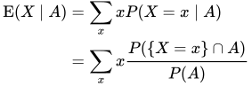
If A is an event in ${\mathcal {F}}$ with nonzero probability, and X is a discrete random variable, the conditional expectation of X given A is

${\begin{aligned}\operatorname {E} (X\mid A)&=\sum _{x}xP(X=x\mid A)\\&=\sum _{x}x{\frac {P(\{X=x\}\cap A)}{P(A)}}\end{aligned}}$

where the sum is taken over all possible outcomes of X.

If $P(A)=0$ , the conditional expectation is undefined due to the division by zero.

Discrete random variables

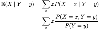
If X and Y are discrete random variables, the conditional expectation of X given Y is

${\begin{aligned}\operatorname {E} (X\mid Y=y)&=\sum _{x}xP(X=x\mid Y=y)\\&=\sum _{x}x{\frac {P(X=x,Y=y)}{P(Y=y)}}\end{aligned}}$

where $P(X=x,Y=y)$ is the joint probability mass function of X and Y. The sum is taken over all possible outcomes of X.

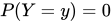
As above, the expression is undefined if $P(Y=y)=0$ .

Conditioning on a discrete random variable is the same as conditioning on the corresponding event:

$\operatorname {E} (X\mid Y=y)=\operatorname {E} (X\mid A)$

where A is the set $\{Y=y\}$ .

Continuous random variables

Let $X$ and $Y$ be continuous random variables with joint density $f_{X,Y}(x,y),$ $Y$ 's density $f_{Y}(y),$ and conditional density $\textstyle f_{X\mid Y}(x\mid y)={\frac {f_{X,Y}(x,y)}{f_{Y}(y)}}$ of $X$ given the event $Y=y.$ The conditional expectation of $X$ given $Y=y$ is

${\begin{aligned}\operatorname {E} (X\mid Y=y)&=\int _{-\infty }^{\infty }xf_{X\mid Y}(x\mid y)\,\mathrm {d} x\\&={\frac {1}{f_{Y}(y)}}\int _{-\infty }^{\infty }xf_{X,Y}(x,y)\,\mathrm {d} x.\end{aligned}}$

When the denominator is zero, the expression is undefined.

Conditioning on a continuous random variable is not the same as conditioning on the event $\{Y=y\}$ as it was in the discrete case. For a discussion, see Conditioning on an event of probability zero. Not respecting this distinction can lead to contradictory conclusions as illustrated by the Borel-Kolmogorov paradox.

L² random variables

All random variables in this section are assumed to be in $L^{2}$ , that is square integrable. In its full generality, conditional expectation is developed without this assumption, see below under Conditional expectation with respect to a sub-σ-algebra. The $L^{2}$ theory is, however, considered more intuitive and admits important generalizations. In the context of $L^{2}$ random variables, conditional expectation is also called regression.

In what follows let $(\Omega ,{\mathcal {F}},P)$ be a probability space, and $X:\Omega \to \mathbb {R}$ in $L^{2}$ with mean $\mu _{X}$ and variance $\sigma _{X}^{2}$ . The expectation $\mu _{X}$ minimizes the mean squared error:

$\min _{x\in \mathbb {R} }\operatorname {E} \left((X-x)^{2}\right)=\operatorname {E} \left((X-\mu _{X})^{2}\right)=\sigma _{X}^{2}.$

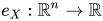
The conditional expectation of X is defined analogously, except instead of a single number $\mu _{X}$ , the result will be a function $e_{X}(y)$ . Let $Y:\Omega \to \mathbb {R} ^{n}$ be a random vector. The conditional expectation $e_{X}:\mathbb {R} ^{n}\to \mathbb {R}$ is a measurable function such that

$\min _{g{\text{ measurable }}}\operatorname {E} \left((X-g(Y))^{2}\right)=\operatorname {E} \left((X-e_{X}(Y))^{2}\right).$

Note that unlike $\mu _{X}$ , the conditional expectation $e_{X}$ is not generally unique: there may be multiple minimizers of the mean squared error.

Uniqueness

Example 1: Consider the case where Y is the constant random variable that is always 1. Then the mean squared error is minimized by any function of the form

$e_{X}(y)={\begin{cases}\mu _{X}&{\text{if }}y=1,\\{\text{any number}}&{\text{otherwise.}}\end{cases}}$

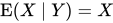
Example 2: Consider the case where Y is the 2-dimensional random vector $(X,2X)$ . Then clearly

$\operatorname {E} (X\mid Y)=X$

but in terms of functions it can be expressed as $e_{X}(y_{1},y_{2})=3y_{1}-y_{2}$ or $e'_{X}(y_{1},y_{2})=y_{2}-y_{1}$ or infinitely many other ways. In the context of linear regression, this lack of uniqueness is called multicollinearity.

Conditional expectation is unique up to a set of measure zero in $\mathbb {R} ^{n}$ . The measure used is the pushforward measure induced by Y.

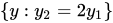
In the first example, the pushforward measure is a Dirac distribution at 1. In the second it is concentrated on the "diagonal" $\{y:y_{2}=2y_{1}\}$ , so that any set not intersecting it has measure 0.

Existence

The existence of a minimizer for $\min _{g}\operatorname {E} \left((X-g(Y))^{2}\right)$ is non-trivial. It can be shown that

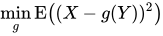
$M:=\{g(Y):g{\text{ is measurable and }}\operatorname {E} (g(Y)^{2})<\infty \}=L^{2}(\Omega ,\sigma (Y))$

is a closed subspace of the Hilbert space $L^{2}(\Omega )$ . By the Hilbert projection theorem, the necessary and sufficient condition for $e_{X}$ to be a minimizer is that for all $f(Y)$ in M we have

$\langle X-e_{X}(Y),f(Y)\rangle =0.$

In words, this equation says that the residual $X-e_{X}(Y)$ is orthogonal to the space M of all functions of Y. This orthogonality condition, applied to the indicator functions $f(Y)=1_{Y\in H}$ , is used below to extend conditional expectation to the case that X and Y are not necessarily in $L^{2}$ .

Connections to regression

The conditional expectation is often approximated in applied mathematics and statistics due to the difficulties in analytically calculating it, and for interpolation.

The Hilbert subspace

$M=\{g(Y):\operatorname {E} (g(Y)^{2})<\infty \}$

defined above is replaced with subsets thereof by restricting the functional form of g, rather than allowing any measurable function. Examples of this are decision tree regression when g is required to be a simple function, linear regression when g is required to be affine, etc.

These generalizations of conditional expectation come at the cost of many of its properties no longer holding. For example, let M be the space of all linear functions of Y and let ${\mathcal {E}}_{M}$ denote this generalized conditional expectation/ $L^{2}$ projection. If $M$ does not contain the constant functions, the tower property $\operatorname {E} ({\mathcal {E}}_{M}(X))=\operatorname {E} (X)$ will not hold.

An important special case is when X and Y are jointly normally distributed. In this case it can be shown that the conditional expectation is equivalent to linear regression:

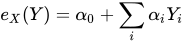
$e_{X}(Y)=\alpha _{0}+\sum _{i}\alpha _{i}Y_{i}$

for coefficients $\{\alpha _{i}\}_{i=0..n}$ described in Multivariate normal distribution#Conditional distributions.

Conditional expectation with respect to a sub-σ-algebra

Consider the following:

$(\Omega ,{\mathcal {F}},P)$ is a probability space.
$X\colon \Omega \to \mathbb {R} ^{n}$ is a random variable on that probability space with finite expectation.
${\mathcal {H}}\subseteq {\mathcal {F}}$ is a sub-σ-algebra of ${\mathcal {F}}$ .

Since ${\mathcal {H}}$ is a sub $\sigma$ -algebra of ${\mathcal {F}}$ , the function $X\colon \Omega \to \mathbb {R} ^{n}$ is usually not ${\mathcal {H}}$ -measurable, thus the existence of the integrals of the form ${\textstyle \int _{H}X\,dP|_{\mathcal {H}}$ , where $H\in {\mathcal {H}}$ and $P|_{\mathcal {H}}$ is the restriction of $P$ to ${\mathcal {H}}$ , cannot be stated in general. However, the local averages ${\textstyle \int _{H}X\,dP$ can be recovered in $(\Omega ,{\mathcal {H}},P|_{\mathcal {H}})$ with the help of the conditional expectation.

A conditional expectation of X given ${\mathcal {H}}$ , denoted as $\operatorname {E} (X\mid {\mathcal {H}})$ , is any ${\mathcal {H}}$ -measurable function $\Omega \to \mathbb {R} ^{n}$ which satisfies:

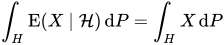
$\int _{H}\operatorname {E} (X\mid {\mathcal {H}})\,\mathrm {d} P=\int _{H}X\,\mathrm {d} P$

for each $H\in {\mathcal {H}}$ .

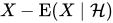
As noted in the $L^{2}$ discussion, this condition is equivalent to saying that the residual $X-\operatorname {E} (X\mid {\mathcal {H}})$ is orthogonal to the indicator functions $1_{H}$ :

$\langle X-\operatorname {E} (X\mid {\mathcal {H}}),1_{H}\rangle =0$

Existence

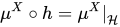
The existence of $\operatorname {E} (X\mid {\mathcal {H}})$ can be established by noting that ${\textstyle \mu ^{X}\colon F\mapsto \int _{F}X\,\mathrm {d} P$ for $F\in {\mathcal {F}}$ is a finite measure on $(\Omega ,{\mathcal {F}})$ that is absolutely continuous with respect to $P$ . If $h$ is the natural injection from ${\mathcal {H}}$ to ${\mathcal {F}}$ , then $\mu ^{X}\circ h=\mu ^{X}|_{\mathcal {H}}$ is the restriction of $\mu ^{X}$ to ${\mathcal {H}}$ and $P\circ h=P|_{\mathcal {H}}$ is the restriction of $P$ to ${\mathcal {H}}$ . Furthermore, $\mu ^{X}\circ h$ is absolutely continuous with respect to $P\circ h$ , because the condition

$P\circ h(H)=0\iff P(h(H))=0$

implies

$\mu ^{X}(h(H))=0\iff \mu ^{X}\circ h(H)=0.$

Thus, we have

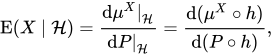
$\operatorname {E} (X\mid {\mathcal {H}})={\frac {\mathrm {d} \mu ^{X}|_{\mathcal {H}}}{\mathrm {d} P|_{\mathcal {H}}}}={\frac {\mathrm {d} (\mu ^{X}\circ h)}{\mathrm {d} (P\circ h)}},$

where the derivatives are Radon-Nikodym derivatives of measures.

Conditional expectation with respect to a random variable

Consider, in addition to the above,

A measurable space $(U,\Sigma )$ , and
A random variable $Y\colon \Omega \to U$ .

The conditional expectation of X given Y is defined by applying the above construction on the σ-algebra generated by Y:

$\operatorname {E} [X\mid Y]:=\operatorname {E} [X\mid \sigma (Y)].$

By the Doob-Dynkin lemma, there exists a measurable function $e_{X}\colon U\to \mathbb {R} ^{n}$ such that

$\operatorname {E} [X\mid Y]=e_{X}(Y).$

Discussion

This is not a constructive definition; we are merely given the required property that a conditional expectation must satisfy.
- The definition of $\operatorname {E} (X\mid {\mathcal {H}})$ may resemble that of $\operatorname {E} (X\mid H)$ for an event $H$ but these are very different objects. The former is a ${\mathcal {H}}$ -measurable function $\Omega \to \mathbb {R} ^{n}$ , while the latter is an element of $\mathbb {R} ^{n}$ and $\operatorname {E} (X\mid H)\ P(H)=\int _{H}X\,\mathrm {d} P=\int _{H}\operatorname {E} (X\mid {\mathcal {H}})\,\mathrm {d} P$ for $H\in {\mathcal {H}}$ .
- Uniqueness can be shown to be almost sure: that is, versions of the same conditional expectation will only differ on a set of probability zero.
  - Often, one would like to think of $\operatorname {E} (X\mid {\mathcal {H}})$ as a measure on $\Omega$ for fixed H. For example, it is extremely useful to claim that $\sum _{i}\operatorname {E} (X_{i}\mid {\mathcal {H}})$ is additive for almost all H. However, this does not immediately follow because each $\operatorname {E} (X_{i}\mid {\mathcal {H}})$ may have a different null set. Because countable unions of null sets are null sets, for a countable set of $X_{i}$ , one can choose "versions" of each $\operatorname {E} (X_{i}\mid {\mathcal {H}})$ with aligned null sets as to maintain additivity for almost all H. However, to align the "null sets of dysfunction" of $\operatorname {E} (X_{i}\mid {\mathcal {H}})$ over all possible $X_{i}$ , and thus treat $\operatorname {E} (X\mid {\mathcal {H}}=H)$ as an almost surely unique measure over $\Omega$ (a "regular probability measure"), we need further regularity conditions. Intuitively, to do this, we need to be able to approximate all possible $X_{i}$ with a countable set of them. This directly corresponds to the conditions for creating a regular probability measure, which are separability and completeness.
The σ-algebra ${\mathcal {H}}$ controls the "granularity" of the conditioning. A conditional expectation $E(X\mid {\mathcal {H}})$ over a finer (larger) σ-algebra ${\mathcal {H}}$ retains information about the probabilities of a larger class of events. A conditional expectation over a coarser (smaller) σ-algebra averages over more events.

Conditional probability

For a Borel subset B in ${\mathcal {B}}(\mathbb {R} ^{n})$ , one can consider the collection of random variables

$\kappa _{\mathcal {H}}(\omega ,B):=\operatorname {E} (1_{X\in B}|{\mathcal {H}})(\omega ).$

It can be shown that they form a Markov kernel, that is, for almost all $\omega$ , $\kappa _{\mathcal {H}}(\omega ,-)$ is a probability measure.

The Law of the unconscious statistician is then

$\operatorname {E} [f(X)\mid {\mathcal {H}}]=\int f(x)\kappa _{\mathcal {H}}(-,\mathrm {d} x),$

This shows that conditional expectations are, like their unconditional counterparts, integrations, against a conditional measure.

General Definition

In full generality, consider:

A probability space $(\Omega ,{\mathcal {A}},P)$ .
A Banach space $(E,\|\cdot \|_{E})$ .
A Bochner integrable random variable $X:\Omega \to E$ .
A sub-σ-algebra ${\mathcal {H}}\subseteq {\mathcal {A}}$ .

The conditional expectation of $X$ given ${\mathcal {H}}$ is the up to a $P$ -nullset unique and integrable $E$ -valued ${\mathcal {H}}$ -measurable random variable $\operatorname {E} (X\mid {\mathcal {H}})$ satisfying

$\int _{H}\operatorname {E} (X\mid {\mathcal {H}})\,\mathrm {d} P=\int _{H}X\,\mathrm {d} P$

for all $H\in {\mathcal {H}}$ .

In this setting the conditional expectation is sometimes also denoted in operator notation as $\operatorname {E} ^{\mathcal {H}}X$ .

04Basic properties

All the following formulas are to be understood in an almost sure sense.

Pulling out independent factors:
- If $X$ is independent of ${\mathcal {H}}$ , then $E(X\mid {\mathcal {H}})=E(X)$ .

Proof

Let $B\in {\mathcal {H}}$ . Then $X$ is independent of $1_{B}$ , so we get that

$\int _{B}X\,dP=E(X1_{B})=E(X)E(1_{B})=E(X)P(B)=\int _{B}E(X)\,dP.$

Thus the definition of conditional expectation is satisfied by the constant random variable $E(X)$ , as desired. $\square$

- If $X$ is independent of $\sigma (Y,{\mathcal {H}})$ , then $E(XY\mid {\mathcal {H}})=E(X)\,E(Y\mid {\mathcal {H}})$ . Note that this is not necessarily the case if $X$ is only independent of ${\mathcal {H}}$ and of $Y$ .
- If $X,Y$ are independent, ${\mathcal {G}},{\mathcal {H}}$ are independent, $X$ is independent of ${\mathcal {H}}$ and $Y$ is independent of ${\mathcal {G}}$ , then $E(E(XY\mid {\mathcal {G}})\mid {\mathcal {H}})=E(X)E(Y)=E(E(XY\mid {\mathcal {H}})\mid {\mathcal {G}})$ .
Stability:
- If $X$ is ${\mathcal {H}}$ -measurable, then $E(X\mid {\mathcal {H}})=X$ .

Proof

For each $H\in {\mathcal {H}}$ we have $\int _{H}E(X\mid {\mathcal {H}})\,dP=\int _{H}X\,dP$ , or equivalently

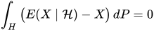
$\int _{H}{\big (}E(X\mid {\mathcal {H}})-X{\big )}\,dP=0$

Since this is true for each $H\in {\mathcal {H}}$ , and both $E(X\mid {\mathcal {H}})$ and $X$ are ${\mathcal {H}}$ -measurable (the former property holds by definition; the latter property is key here), from this one can show

$\int _{H}{\big |}E(X\mid {\mathcal {H}})-X{\big |}\,dP=0$

And this implies $E(X\mid {\mathcal {H}})=X$ almost everywhere. $\square$

- In particular, for sub-σ-algebras ${\mathcal {H}}_{1}\subset {\mathcal {H}}_{2}\subset {\mathcal {F}}$ we have $E(E(X\mid {\mathcal {H}}_{1})\mid {\mathcal {H}}_{2})=E(X\mid {\mathcal {H}}_{1})$ . (Note this is different from the tower property below.)
- If Z is a random variable, then $\operatorname {E} (f(Z)\mid Z)=f(Z)$ . In its simplest form, this says $\operatorname {E} (Z\mid Z)=Z$ .
Pulling out known factors:
- If $X$ is ${\mathcal {H}}$ -measurable, then $E(XY\mid {\mathcal {H}})=X\,E(Y\mid {\mathcal {H}})$ .

Proof

All random variables here are assumed without loss of generality to be non-negative. The general case can be treated with $X=X^{+}-X^{-}$ .

Fix $A\in {\mathcal {H}}$ and let $X=1_{A}$ . Then for any $H\in {\mathcal {H}}$

$\int _{H}E(1_{A}Y\mid {\mathcal {H}})\,dP=\int _{H}1_{A}Y\,dP=\int _{A\cap H}Y\,dP=\int _{A\cap H}E(Y\mid {\mathcal {H}})\,dP=\int _{H}1_{A}E(Y\mid {\mathcal {H}})\,dP$

Hence $E(1_{A}Y\mid {\mathcal {H}})=1_{A}E(Y\mid {\mathcal {H}})$ almost everywhere.

Any simple function is a finite linear combination of indicator functions. By linearity the above property holds for simple functions: if $X_{n}$ is a simple function then $E(X_{n}Y\mid {\mathcal {H}})=X_{n}\,E(Y\mid {\mathcal {H}})$ .

Now let $X$ be ${\mathcal {H}}$ -measurable. Then there exists a sequence of simple functions $\{X_{n}\}_{n\geq 1}$ converging monotonically (here meaning $X_{n}\leq X_{n+1}$ ) and pointwise to $X$ . Consequently, for $Y\geq 0$ , the sequence $\{X_{n}Y\}_{n\geq 1}$ converges monotonically and pointwise to $XY$ .

Also, since $E(Y\mid {\mathcal {H}})\geq 0$ , the sequence $\{X_{n}E(Y\mid {\mathcal {H}})\}_{n\geq 1}$ converges monotonically and pointwise to $X\,E(Y\mid {\mathcal {H}})$

Combining the special case proved for simple functions, the definition of conditional expectation, and deploying the monotone convergence theorem:

$\int _{H}X\,E(Y\mid {\mathcal {H}})\,dP=\int _{H}\lim _{n\to \infty }X_{n}\,E(Y\mid {\mathcal {H}})\,dP=\lim _{n\to \infty }\int _{H}X_{n}E(Y\mid {\mathcal {H}})\,dP=\lim _{n\to \infty }\int _{H}E(X_{n}Y\mid {\mathcal {H}})\,dP=\lim _{n\to \infty }\int _{H}X_{n}Y\,dP=\int _{H}\lim _{n\to \infty }X_{n}Y\,dP=\int _{H}XY\,dP=\int _{H}E(XY\mid {\mathcal {H}})\,dP$

This holds for all $H\in {\mathcal {H}}$ , whence $X\,E(Y\mid {\mathcal {H}})=E(XY\mid {\mathcal {H}})$ almost everywhere. $\square$

- If Z is a random variable, then $\operatorname {E} (f(Z)Y\mid Z)=f(Z)\operatorname {E} (Y\mid Z)$ .
Law of total expectation: $E(E(X\mid {\mathcal {H}}))=E(X)$ .
Tower property:
- For sub-σ-algebras we have .
  - A special case ${\mathcal {H}}_{1}=\{\emptyset ,\Omega \}$ recovers the Law of total expectation: $E(E(X\mid {\mathcal {H}}_{2}))=E(X)$ .
  - A special case is when Z is a ${\mathcal {H}}$ -measurable random variable. Then $\sigma (Z)\subset {\mathcal {H}}$ and thus $E(E(X\mid {\mathcal {H}})\mid Z)=E(X\mid Z)$ .
  - Doob martingale property: the above with $Z=E(X\mid {\mathcal {H}})$ (which is ${\mathcal {H}}$ -measurable), and using also $\operatorname {E} (Z\mid Z)=Z$ , gives $E(X\mid E(X\mid {\mathcal {H}}))=E(X\mid {\mathcal {H}})$ .
- For random variables $X,Y$ we have $E(E(X\mid Y)\mid f(Y))=E(X\mid f(Y))$ .
- For random variables $X,Y,Z$ we have $E(E(X\mid Y,Z)\mid Y)=E(X\mid Y)$ .
Linearity: we have $E(X_{1}+X_{2}\mid {\mathcal {H}})=E(X_{1}\mid {\mathcal {H}})+E(X_{2}\mid {\mathcal {H}})$ and $E(aX\mid {\mathcal {H}})=a\,E(X\mid {\mathcal {H}})$ for $a\in \mathbb {R}$ .
Positivity: If $X\geq 0$ then $E(X\mid {\mathcal {H}})\geq 0$ .
Monotonicity: If $X_{1}\leq X_{2}$ then $E(X_{1}\mid {\mathcal {H}})\leq E(X_{2}\mid {\mathcal {H}})$ .
Monotone convergence: If $0\leq X_{n}\uparrow X$ then $E(X_{n}\mid {\mathcal {H}})\uparrow E(X\mid {\mathcal {H}})$ .
Dominated convergence: If $X_{n}\to X$ and $|X_{n}|\leq Y$ with $Y\in L^{1}$ , then $E(X_{n}\mid {\mathcal {H}})\to E(X\mid {\mathcal {H}})$ .
Fatou's lemma: If $\textstyle E(\inf _{n}X_{n}\mid {\mathcal {H}})>-\infty$ then $\textstyle E(\liminf _{n\to \infty }X_{n}\mid {\mathcal {H}})\leq \liminf _{n\to \infty }E(X_{n}\mid {\mathcal {H}})$ .
Jensen's inequality: If $f\colon \mathbb {R} \rightarrow \mathbb {R}$ is a convex function, then $f(E(X\mid {\mathcal {H}}))\leq E(f(X)\mid {\mathcal {H}})$ .
Conditional variance: Using the conditional expectation we can define, by analogy with the definition of the variance as the mean square deviation from the average, the conditional variance
- Definition: $\operatorname {Var} (X\mid {\mathcal {H}})=\operatorname {E} {\bigl (}(X-\operatorname {E} (X\mid {\mathcal {H}}))^{2}\mid {\mathcal {H}}{\bigr )}$
- Algebraic formula for the variance: $\operatorname {Var} (X\mid {\mathcal {H}})=\operatorname {E} (X^{2}\mid {\mathcal {H}})-{\bigl (}\operatorname {E} (X\mid {\mathcal {H}}){\bigr )}^{2}$
- Law of total variance: $\operatorname {Var} (X)=\operatorname {E} (\operatorname {Var} (X\mid {\mathcal {H}}))+\operatorname {Var} (\operatorname {E} (X\mid {\mathcal {H}}))$ .
Martingale convergence: For a random variable $X$ , that has finite expectation, we have $E(X\mid {\mathcal {H}}_{n})\to E(X\mid {\mathcal {H}})$ , if either ${\mathcal {H}}_{1}\subset {\mathcal {H}}_{2}\subset \dotsb$ is an increasing series of sub-σ-algebras and $\textstyle {\mathcal {H}}=\sigma (\bigcup _{n=1}^{\infty }{\mathcal {H}}_{n})$ or if ${\mathcal {H}}_{1}\supset {\mathcal {H}}_{2}\supset \dotsb$ is a decreasing series of sub-σ-algebras and $\textstyle {\mathcal {H}}=\bigcap _{n=1}^{\infty }{\mathcal {H}}_{n}$ .
Conditional expectation as -projection: If are in the Hilbert space of square-integrable real random variables (real random variables with finite second moment) then
- for ${\mathcal {H}}$ -measurable $Y$ , we have $E(Y(X-E(X\mid {\mathcal {H}})))=0$ , i.e. the conditional expectation $E(X\mid {\mathcal {H}})$ is in the sense of the L²(P) scalar product the orthogonal projection from $X$ to the linear subspace of ${\mathcal {H}}$ -measurable functions. (This allows to define and prove the existence of the conditional expectation based on the Hilbert projection theorem.)
- the mapping $X\mapsto \operatorname {E} (X\mid {\mathcal {H}})$ is self-adjoint: $\operatorname {E} (X\operatorname {E} (Y\mid {\mathcal {H}}))=\operatorname {E} \left(\operatorname {E} (X\mid {\mathcal {H}})\operatorname {E} (Y\mid {\mathcal {H}})\right)=\operatorname {E} (\operatorname {E} (X\mid {\mathcal {H}})Y)$
Conditioning is a contractive projection of L^p spaces $L^{p}(\Omega ,{\mathcal {F}},P)\rightarrow L^{p}(\Omega ,{\mathcal {H}},P)$ . I.e., $\operatorname {E} {\big (}|\operatorname {E} (X\mid {\mathcal {H}})|^{p}{\big )}\leq \operatorname {E} {\big (}|X|^{p}{\big )}$ for any p ≥ 1.
Doob's conditional independence property: If $X,Y$ are conditionally independent given $Z$ , then $P(X\in B\mid Y,Z)=P(X\in B\mid Z)$ (equivalently, $E(1_{\{X\in B\}}\mid Y,Z)=E(1_{\{X\in B\}}\mid Z)$ ).

Watch videos about Conditional expectationExplainers and documentaries on YouTube (opens in a new tab)

Sources and credits

This article is adapted from the Wikipedia article “Conditional expectation”, written by its contributors and licensed under CC BY-SA 4.0. Fathomly has changed the layout, removed citation markers, navigation and maintenance notices, and adjusted punctuation. This adapted version is shared under the same license. For references, see the original article.

Images, from Wikimedia Commons:

LokaleMittelwertbildung.svg by Erzbischof, CC BY-SA 3.0

Fathomly is not affiliated with or endorsed by the Wikimedia Foundation. Spotted a problem? Tell us.

Conditional expectation

01Examples

Example 1: Dice rolling

Example 2: Rainfall data

02History

03Definitions

Conditioning on an event

Discrete random variables

Continuous random variables

L² random variables

Uniqueness

Existence

Connections to regression

Conditional expectation with respect to a sub-σ-algebra

Existence

Conditional expectation with respect to a random variable

Discussion

Conditional probability

General Definition

04Basic properties

Sources and credits

Related topics

Conditioning (probability)

Disintegration theorem

Doob-Dynkin lemma

Conditional expectation

01Examples

Example 1: Dice rolling

Example 2: Rainfall data

02History

03Definitions

Conditioning on an event

Discrete random variables

Continuous random variables

L2 random variables

Uniqueness

Existence

Connections to regression

Conditional expectation with respect to a sub-σ-algebra

Existence

Conditional expectation with respect to a random variable

Discussion

Conditional probability

General Definition

04Basic properties

Sources and credits

Related topics

Conditioning (probability)

Disintegration theorem

Doob-Dynkin lemma

L² random variables