Expected shortfall
Risk measure estimating the average loss in the worst tail of the distribution
Expected shortfall (ES) is a risk measure, a concept used in the field of financial risk measurement to evaluate the market risk or credit risk of a portfolio. The "expected shortfall at q% level" is the expected return on the portfolio in the worst 
Expected shortfall is also called conditional value at risk (CVaR), average value at risk (AVaR), tail value at risk (TVaR), conditional tail expectation (CTE), expected tail loss (ETL), and superquantile. These names are often used interchangeably, although several definitions exist in the literature. These definitions coincide in many cases, but may differ for certain types of loss distributions.
01Background
Risk measures are used both in mathematical finance and in actuarial science, and the value-at-risk and expected shortfall measures are often expressed using different sign conventions and tail conventions in these disciplines. The discussion that follows takes the mathematical finance point of view.
In mathematical finance, risk measures arise when considering the profit/loss distribution, i.e., payoff, for a financial portfolio, modeled as a random variable 

![\alpha \in [0,1]](https://wikimedia.org/api/rest_v1/media/math/render/svg/daf3c62599ea71319c85f715c9e590d2bab2d036)


![[0,\alpha ]](https://wikimedia.org/api/rest_v1/media/math/render/svg/fe67ac673f6464193d5ee8c6e721963a55702b97)
Expected shortfall is often considered preferable to VaR because it accounts for the severity of the failure, not only the chance of failure. Further, it is a coherent spectral measure of financial portfolio risk, while VaR is not. This is a collection of mathematical properties, one of which ensures that diversification of a portfolio never leads to a higher measure of risk. Viewing the value produced by a risk measure as a capital reserve requirement, ES at level
02Formal definition
If 

where 
Several other definitions appear in the literature under the names ES, TVaR, AVaR, CTE, and CVaR. The formulation above as an integral of VaR values is coherent and well-defined in the general case. Other definitions typically coincide under common assumptions such as continuity of the loss distribution, but may differ for distributions with atoms.
The above definition is equivalent to
![\operatorname {ES} _{\alpha }(X)=-{\frac {1}{\alpha }}\left(\operatorname {E} [X\ 1_{\{X\leq x_{\alpha }\}}]+x_{\alpha }(\alpha -P[X\leq x_{\alpha }])\right)](https://wikimedia.org/api/rest_v1/media/math/render/svg/4b3aaa61637c82ae386cdac3fbccc3a96432eb94)
where 
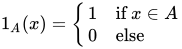
Some authors define expected shortfall, tail conditional expectation, or related quantities directly as a conditional expectation beyond the relevant quantile,
![\operatorname {ES} _{\alpha }(X)=-E[X|X<x_{\alpha }]](https://wikimedia.org/api/rest_v1/media/math/render/svg/e2c582e65bdea57e480c7f86781e4427a24d46b4)
This formulation agrees with the general definition above when the distribution is continuous at 
Some variation in definitions arise from the differing conventions used between, say, financial mathematics and actuarial science, where things written with one set of conventions can be translated into a context with different ones. But there is further inconsistency, with some cases of substantively different definitions used for the same term. For instance, Sweeting defines TVaR as the tail conditional expectation, whereas he defines expected shortfall as the scaled version 
There are a number of related, but subtly different, formulations for TVaR in the literature. A common case in literature is to define TVaR and average value at risk as the same measure. Under some formulations, it is only equivalent to expected shortfall when the underlying distribution function is continuous at
The canonical tail value at risk is the left-tail (large negative values) in some disciplines and the right-tail (large positive values) in other, such as actuarial science. This is usually due to the differing conventions of treating losses as large negative or positive values. Using the negative value convention, Artzner and others define the tail value at risk as:
Given a random variable 
![\operatorname {TVaR} _{\alpha }(X)=\operatorname {E} [-X|X\leq -\operatorname {VaR} _{\alpha }(X)]=\operatorname {E} [-X|X\leq x^{\alpha }],](https://wikimedia.org/api/rest_v1/media/math/render/svg/9a43fcb4528aea744af04aaa030d657a563acd40)



The dual representation is
![\operatorname {ES} _{\alpha }(X)=\inf _{Q\in {\mathcal {Q}}_{\alpha }}E^{Q}[X]](https://wikimedia.org/api/rest_v1/media/math/render/svg/10ae29b404213dc3ca11c18bd04acd98c6db1558)
where 


Expected shortfall can be generalized to a general class of coherent risk measures on 

If the underlying distribution for ![\operatorname {TCE} _{\alpha }(X)=E[-X\mid X\leq -\operatorname {VaR} _{\alpha }(X)]](https://wikimedia.org/api/rest_v1/media/math/render/svg/4f2e31467cc3e105f118448bb98a91f2d20898c4)
Informally, and non-rigorously, this equation amounts to saying "in case of losses so severe that they occur only alpha percent of the time, what is our average loss".
Expected shortfall can also be written as a distortion risk measure given by the distortion function

03Examples
Example 1. If we believe our average loss on the worst 5% of the possible outcomes for our portfolio is EUR 1000, then we could say our expected shortfall is EUR 1000 for the 5% tail.
Example 2. Consider a portfolio that will have the following possible values at the end of the period:
| probability of event |
ending value of the portfolio |
|---|---|
| 10% | 0 |
| 30% | 80 |
| 40% | 100 |
| 20% | 150 |
Now assume that we paid 100 at the beginning of the period for this portfolio. Then the profit in each case is (ending value−100) or:
| probability of event |
profit |
|---|---|
| 10% | −100 |
| 30% | −20 |
| 40% | 0 |
| 20% | 50 |
From this table let us calculate the expected shortfall 

|
expected shortfall |
|---|---|
| 5% | 100 |
| 10% | 100 |
| 20% | 60 |
| 30% | 46.6 |
| 40% | 40 |
| 50% | 32 |
| 60% | 26.6 |
| 80% | 20 |
| 90% | 12.2 |
| 100% | 6 |
To see how these values were calculated, consider the calculation of 
Now consider the calculation of 
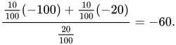
Similarly for any value of 
As a final example, calculate 

The value at risk (VaR) is given below for comparison.
|
 |
|---|---|
 |
100 |
 |
20 |
 |
0 |
 |
-50 |
04Properties
The expected shortfall
The 100%-quantile expected shortfall 
For a given portfolio, the expected shortfall
05Optimization of expected shortfall
Expected shortfall, in its standard form, is known to lead to a generally non-convex optimization problem. However, it is possible to transform the problem into a linear program and find the global solution. This property makes expected shortfall a cornerstone of alternatives to mean-variance portfolio optimization, which account for the higher moments (e.g., skewness and kurtosis) of a return distribution.
Suppose that we want to minimize the expected shortfall of a portfolio. The key contribution of Rockafellar and Uryasev in their 2000 paper is to introduce the auxiliary function 
![F_{\alpha }(w,\gamma )=\gamma +{1 \over {1-\alpha }}\int _{\ell (w,x)\geq \gamma }\left[\ell (w,x)-\gamma \right]_{+}p(x)\,dx](https://wikimedia.org/api/rest_v1/media/math/render/svg/47c333469bb086740e6079f6e3bb99f6ea453ab6)
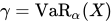


![{\widetilde {F}}_{\alpha }(w,\gamma )=\gamma +{1 \over {(1-\alpha )J}}\sum _{j=1}^{J}[\ell (w,x_{j})-\gamma ]_{+}](https://wikimedia.org/api/rest_v1/media/math/render/svg/e64bb51899eb5feb3302a32b44cfe1aa419a232e)


06Formulas for continuous probability distributions
Closed-form formulas exist for calculating the expected shortfall when the payoff of a portfolio 

![\operatorname {ES} _{\alpha }(X)=E[-X\mid X\leq -\operatorname {VaR} _{\alpha }(X)]=-{\frac {1}{\alpha }}\int _{0}^{\alpha }\operatorname {VaR} _{\gamma }(X)\,d\gamma =-{\frac {1}{\alpha }}\int _{-\infty }^{-\operatorname {VaR} _{\alpha }(X)}xf(x)\,dx.](https://wikimedia.org/api/rest_v1/media/math/render/svg/b27d5a69ce9afd5b0b7ddc51ec4c19aa7b3daea8)
Typical values of 
For engineering or actuarial applications it is more common to consider the distribution of losses 
![\operatorname {ES} _{\alpha }(L)=\operatorname {E} [L\mid L\geq \operatorname {VaR} _{\alpha }(L)]={\frac {1}{1-\alpha }}\int _{\alpha }^{1}\operatorname {VaR} _{\gamma }(L)\,d\gamma ={\frac {1}{1-\alpha }}\int _{\operatorname {VaR} _{\alpha }(L)}^{+\infty }yf(y)\,dy.](https://wikimedia.org/api/rest_v1/media/math/render/svg/fbc45340ee7d389f415b65a94d1c0358b677a40f)
Since some formulas below were derived for the left-tail case and some for the right-tail case, the following reconciliations can be useful:
![\operatorname {ES} _{\alpha }(X)=-{\frac {1}{\alpha }}\operatorname {E} [X]+{\frac {1-\alpha }{\alpha }}\operatorname {ES} _{\alpha }(L){\text{ and }}\operatorname {ES} _{\alpha }(L)={\frac {1}{1-\alpha }}\operatorname {E} [L]+{\frac {\alpha }{1-\alpha }}\operatorname {ES} _{\alpha }(X).](https://wikimedia.org/api/rest_v1/media/math/render/svg/c592f4db6c9c77e3b74e4c34ea60597b565e9edb)
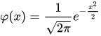
Normal distribution
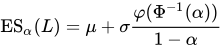
If the payoff of a portfolio 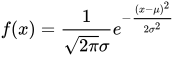



If the loss of a portfolio 
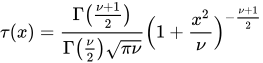
Generalized Student's t-distribution
If the payoff of a portfolio 



If the loss of a portfolio 
Laplace distribution
If the payoff of a portfolio
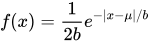
and the c.d.f.
![F(x)={\begin{cases}1-{\frac {1}{2}}e^{-(x-\mu )/b}&{\text{if }}x\geq \mu ,\\[4pt]{\frac {1}{2}}e^{(x-\mu )/b}&{\text{if }}x<\mu .\end{cases}}](https://wikimedia.org/api/rest_v1/media/math/render/svg/5bc74653846f1e6243ac2db148976eee1393f69e)
then the expected shortfall is equal to 

If the loss of a portfolio
![\operatorname {ES} _{\alpha }(L)={\begin{cases}\mu +b{\frac {\alpha }{1-\alpha }}(1-\ln 2\alpha )&{\text{if }}\alpha <0.5,\\[4pt]\mu +b[1-\ln(2(1-\alpha ))]&{\text{if }}\alpha \geq 0.5.\end{cases}}](https://wikimedia.org/api/rest_v1/media/math/render/svg/d84aa79aa5d69bffbaf45a3a9bbaa69ef8869cfa)
Logistic distribution
If the payoff of a portfolio 
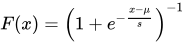

If the loss of a portfolio 
Exponential distribution
If the loss of a portfolio 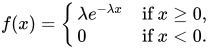
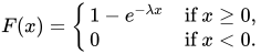
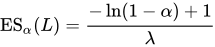
Pareto distribution
If the loss of a portfolio 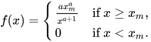


Generalized Pareto distribution (GPD)
If the loss of a portfolio
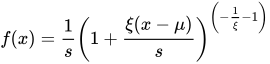
and the c.d.f.
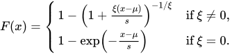
then the expected shortfall is equal to
![\operatorname {ES} _{\alpha }(L)={\begin{cases}\mu +s\left[{\frac {(1-\alpha )^{-\xi }}{1-\xi }}+{\frac {(1-\alpha )^{-\xi }-1}{\xi }}\right]&{\text{if }}\xi \neq 0,\\\mu +s\left[1-\ln(1-\alpha )\right]&{\text{if }}\xi =0,\end{cases}}](https://wikimedia.org/api/rest_v1/media/math/render/svg/0828a7a99120dab1446bec19bb757238104c3aca)
and the VaR is equal to

Weibull distribution
If the loss of a portfolio 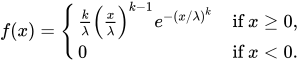



Generalized extreme value distribution (GEV)
If the payoff of a portfolio ![f(x)={\begin{cases}{\frac {1}{\sigma }}\left(1+\xi {\frac {x-\mu }{\sigma }}\right)^{-{\frac {1}{\xi }}-1}\exp \left[-\left(1+\xi {\frac {x-\mu }{\sigma }}\right)^{-{1}/{\xi }}\right]&{\text{if }}\xi \neq 0,\\{\frac {1}{\sigma }}e^{-{\frac {x-\mu }{\sigma }}}e^{-e^{-{\frac {x-\mu }{\sigma }}}}&{\text{if }}\xi =0.\end{cases}}](https://wikimedia.org/api/rest_v1/media/math/render/svg/79cbe26f052efc3c54b8f6d02b8aa5afd4ef078b)
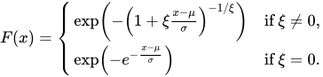
![\operatorname {ES} _{\alpha }(X)={\begin{cases}-\mu -{\frac {\sigma }{\alpha \xi }}{\big [}\Gamma (1-\xi ,-\ln \alpha )-\alpha {\big ]}&{\text{if }}\xi \neq 0,\\-\mu -{\frac {\sigma }{\alpha }}{\big [}{\text{li}}(\alpha )-\alpha \ln(-\ln \alpha ){\big ]}&{\text{if }}\xi =0.\end{cases}}](https://wikimedia.org/api/rest_v1/media/math/render/svg/21061bead9239e58dbcc0e54072d89bcdd3952da)
![\operatorname {VaR} _{\alpha }(X)={\begin{cases}-\mu -{\frac {\sigma }{\xi }}\left[(-\ln \alpha )^{-\xi }-1\right]&{\text{if }}\xi \neq 0,\\-\mu +\sigma \ln(-\ln \alpha )&{\text{if }}\xi =0.\end{cases}}](https://wikimedia.org/api/rest_v1/media/math/render/svg/f10aba4a9f218313a0c650da068975d6d04f6bb8)

If the loss of a portfolio ![\operatorname {ES} _{\alpha }(X)={\begin{cases}\mu +{\frac {\sigma }{(1-\alpha )\xi }}{\bigl [}\gamma (1-\xi ,-\ln \alpha )-(1-\alpha ){\bigr ]}&{\text{if }}\xi \neq 0,\\\mu +{\frac {\sigma }{1-\alpha }}{\bigl [}y-{\text{li}}(\alpha )+\alpha \ln(-\ln \alpha ){\bigr ]}&{\text{if }}\xi =0.\end{cases}}](https://wikimedia.org/api/rest_v1/media/math/render/svg/a2dba415ffd035b872dd7d1b9fc8c7c263a04112)


Generalized hyperbolic secant (GHS) distribution
If the payoff of a portfolio 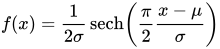
![F(x)={\frac {2}{\pi }}\arctan \left[\exp \left({\frac {\pi }{2}}{\frac {x-\mu }{\sigma }}\right)\right]](https://wikimedia.org/api/rest_v1/media/math/render/svg/40e0860eb7b66ecfc89b2e501511351c1615ffc5)
![\operatorname {ES} _{\alpha }(X)=-\mu -{\frac {2\sigma }{\pi }}\ln \left(\tan {\frac {\pi \alpha }{2}}\right)-{\frac {2\sigma }{\pi ^{2}\alpha }}i\left[\operatorname {Li} _{2}\left(-i\tan {\frac {\pi \alpha }{2}}\right)-\operatorname {Li} _{2}\left(i\tan {\frac {\pi \alpha }{2}}\right)\right]](https://wikimedia.org/api/rest_v1/media/math/render/svg/8d2f3cf358635c87055b57e48c565b31950f5731)


Johnson's SU-distribution
If the payoff of a portfolio ![F(x)=\Phi \left[\gamma +\delta \sinh ^{-1}\left({\frac {x-\xi }{\lambda }}\right)\right]](https://wikimedia.org/api/rest_v1/media/math/render/svg/bc71f4b7428dc370287f5ef90249a0bd2eb86b75)
![\operatorname {ES} _{\alpha }(X)=-\xi -{\frac {\lambda }{2\alpha }}\left[\exp \left({\frac {1-2\gamma \delta }{2\delta ^{2}}}\right)\;\Phi \left(\Phi ^{-1}(\alpha )-{\frac {1}{\delta }}\right)-\exp \left({\frac {1+2\gamma \delta }{2\delta ^{2}}}\right)\;\Phi \left(\Phi ^{-1}(\alpha )+{\frac {1}{\delta }}\right)\right]](https://wikimedia.org/api/rest_v1/media/math/render/svg/4e6020b35cc8398cc34e1d60602e16c607e06d60)

Burr type XII distribution
If the payoff of a portfolio ![f(x)={\frac {ck}{\beta }}\left({\frac {x-\gamma }{\beta }}\right)^{c-1}\left[1+\left({\frac {x-\gamma }{\beta }}\right)^{c}\right]^{-k-1}](https://wikimedia.org/api/rest_v1/media/math/render/svg/016c07ff59be5fcb9e0118727745b0a82f5883ea)
![F(x)=1-\left[1+\left({\frac {x-\gamma }{\beta }}\right)^{c}\right]^{-k}](https://wikimedia.org/api/rest_v1/media/math/render/svg/3aa018db567f5b024ee135f816c3fb735527c9e7)
![\operatorname {ES} _{\alpha }(X)=-\gamma -{\frac {\beta }{\alpha }}\left((1-\alpha )^{-1/k}-1\right)^{1/c}\left[\alpha -1+{_{2}F_{1}}\left({\frac {1}{c}},k;1+{\frac {1}{c}};1-(1-\alpha )^{-1/k}\right)\right]](https://wikimedia.org/api/rest_v1/media/math/render/svg/91683a8cdde99bac106695c9bdb270ce5d056296)


Dagum distribution
If the payoff of a portfolio ![f(x)={\frac {ck}{\beta }}\left({\frac {x-\gamma }{\beta }}\right)^{ck-1}\left[1+\left({\frac {x-\gamma }{\beta }}\right)^{c}\right]^{-k-1}](https://wikimedia.org/api/rest_v1/media/math/render/svg/2156ace29c273bacd1a301ff8dea896df993e187)
![F(x)=\left[1+\left({\frac {x-\gamma }{\beta }}\right)^{-c}\right]^{-k}](https://wikimedia.org/api/rest_v1/media/math/render/svg/fcaf5ae59f211cffd7eb9303a8f050ed551700d4)

Lognormal distribution
If the payoff of a portfolio 

Log-logistic distribution
If the payoff of a portfolio 

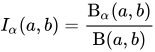
As the incomplete beta function is defined only for positive arguments, for a more generic case the expected shortfall can be expressed with the hypergeometric function: 
If the loss of a portfolio 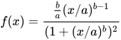
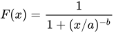
![\operatorname {ES} _{\alpha }(L)={\frac {a}{1-\alpha }}\left[{\frac {\pi }{b}}\csc \left({\frac {\pi }{b}}\right)-\mathrm {B} _{\alpha }\left({\frac {1}{b}}+1,1-{\frac {1}{b}}\right)\right]](https://wikimedia.org/api/rest_v1/media/math/render/svg/187489f78049d447826f6c7da5a49b7f54bdd4c2)

Log-Laplace distribution
If the payoff of a portfolio 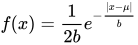
![\operatorname {ES} _{\alpha }(X)={\begin{cases}1-{\frac {e^{\mu }(2\alpha )^{b}}{b+1}}&{\text{if }}\alpha \leq 0.5,\\1-{\frac {e^{\mu }2^{-b}}{\alpha (b-1)}}\left[(1-\alpha )^{(1-b)}-1\right]&{\text{if }}\alpha >0.5.\end{cases}}](https://wikimedia.org/api/rest_v1/media/math/render/svg/b7b484d9d7dc9a5719e04ed634fd9d49f934c819)
Log-generalized hyperbolic secant (log-GHS) distribution
If the payoff of a portfolio

where
07Dynamic expected shortfall
The conditional version of the expected shortfall at the time t is defined by
![\operatorname {ES} _{\alpha }^{t}(X)=\operatorname {ess\sup } _{Q\in {\mathcal {Q}}_{\alpha }^{t}}E^{Q}[-X\mid {\mathcal {F}}_{t}]](https://wikimedia.org/api/rest_v1/media/math/render/svg/0987e7687617fddd3dd4319ba647d4edab3306d5)
where 
This is not a time-consistent risk measure. The time-consistent version is given by
![\rho _{\alpha }^{t}(X)=\operatorname {ess\sup } _{Q\in {\tilde {\mathcal {Q}}}_{\alpha }^{t}}E^{Q}[-X\mid {\mathcal {F}}_{t}]](https://wikimedia.org/api/rest_v1/media/math/render/svg/eb5535550562e8131fb6f5a5a429e81b01c67b8c)
such that
![{\tilde {\mathcal {Q}}}_{\alpha }^{t}=\left\{Q\ll P:\operatorname {E} \left[{\frac {dQ}{dP}}\mid {\mathcal {F}}_{\tau +1}\right]\leq \alpha _{t}^{-1}\operatorname {E} \left[{\frac {dQ}{dP}}\mid {\mathcal {F}}_{\tau }\right]\;\forall \tau \geq t{\text{ a.s.}}\right\}.](https://wikimedia.org/api/rest_v1/media/math/render/svg/1e138fe00e7a6f9a28f21275aa95b520cb312e7c)
Sources and credits
This article is adapted from the Wikipedia article “Expected shortfall”, written by its contributors and licensed under CC BY-SA 4.0. Fathomly has changed the layout, removed citation markers, navigation and maintenance notices, and adjusted punctuation. This adapted version is shared under the same license. For references, see the original article.
Fathomly is not affiliated with or endorsed by the Wikimedia Foundation. Spotted a problem? Tell us.