Encyclopedia

Wiener process

Stochastic process generalizing Brownian motion

Wikipedia contributorsAdapted for Fathomly · View authors

20 min read
Source updated September 5, 2026

In mathematics, the Wiener process (or Brownian motion, due to its historical connection with the physical process of the same name) is a real-valued continuous-time stochastic process named after Norbert Wiener. It is one of the best known Lévy processes (càdlàg stochastic processes with stationary independent increments). It occurs frequently in pure and applied mathematics, economics, quantitative finance, evolutionary biology, and physics.

The Wiener process plays an important role in both pure and applied mathematics. In pure mathematics, the Wiener process gave rise to the study of continuous time martingales. It is a key process in terms of which more complicated stochastic processes can be described. As such, it plays a vital role in stochastic calculus, diffusion processes and even potential theory. It is the driving process of Schramm-Loewner evolution. In applied mathematics, the Wiener process is used to represent the integral of a white noise Gaussian process, and so is useful as a model of noise in electronics engineering (see Brownian noise), instrument errors in filtering theory and disturbances in control theory.

The Wiener process has applications throughout the mathematical sciences. In physics, researchers use it to model Brownian motion and other types of diffusion, often through the Fokker-Planck and Langevin equations, which describe how random motion evolves over time. It also underpins the rigorous path integral formulation of quantum mechanics: by the Feynman-Kac formula, one can represent solutions to the Schrödinger equation in terms of the Wiener process. In physical cosmology, it also appears in models of eternal inflation. The Wiener process is prominent in the mathematical theory of finance as well, in particular the Black-Scholes option pricing model.

01Definitions

Canonical definition

The Wiener process W is a real-valued continuous-time stochastic process characterized by the following properties:

W₀ = 0 almost surely.
W has independent increments: for every t > 0, the future increments ${\textstyle W_{t+u}-W_{t},\,u>0,$ are independent of the past values W_s, s < t. Equivalently, for every t > 0 and ${\textstyle u\geq 0$ , the increment ${\textstyle W_{t+u}-W_{t}$ is independent of the sigma-algebra ${\textstyle {\mathcal {F}}_{t}^{B}=\sigma (W_{s}:0\leq s\leq t)$ .
W has Gaussian increments: for all ${\textstyle u,t\geq 0$ , ${\textstyle W_{t+u}-W_{t}\sim {\mathcal {N}}(0,u).$ That is, a time step u results in an increment that is normally distributed with mean 0 and variance u.
W has almost surely continuous paths: W_t is almost surely continuous in t.

That the process has independent increments means that if 0 ≤ s₁ < t₁ ≤ s₂ < t₂ then W_t₁ − W_s₁ and W_t₂ − W_s₂ are independent random variables, and the similar condition holds for n increments.

The Wiener measure is the probability law of the Wiener process on the space of continuous functions g with g(0) = 0 equipped with the Borel σ-algebra. An integral with respect to the Wiener measure may be called a Wiener integral.

Lévy characterization

An alternative characterization of the Wiener process is the so-called Lévy characterization: A continuous (local) martingale W with W₀ = 0 is a Wiener process if and only if its quadratic variation is [W, W]_t = t (which means that W_t² − t is a (local) martingale).

Gaussian process characterization

The Wiener process can be equivalently defined as a Gaussian process $W_{t}$ , that is, a stochastic process such that for every set of indices $t_{1},\dots ,t_{n}\geq 0$ , the random vector $(W_{t_{1}},\dots ,W_{t_{n}})$ is multivariate Gaussian, which has continuous paths and such that for all $s,t\geq 0$ it holds

${\begin{aligned}&\operatorname {E} [W_{t}]=0,\\&\mathrm {Cov} (W_{t},W_{s})=\operatorname {E} [W_{s}W_{t}]=\min(s,t).\end{aligned}}$

In particular, the law of $W$ on the space of continuous functions (equipped with the Borel σ-algebra) is uniquely determined, which is the Wiener measure.

Wiener representation

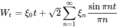
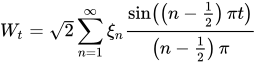
Wiener (1923) also gave a representation of a Brownian path in terms of a random Fourier series. If ${\textstyle \xi _{n}$ are independent Gaussian variables with mean zero and variance one, then $W_{t}=\xi _{0}t+{\sqrt {2}}\sum _{n=1}^{\infty }\xi _{n}{\frac {\sin \pi nt}{\pi n}}$ and $W_{t}={\sqrt {2}}\sum _{n=1}^{\infty }\xi _{n}{\frac {\sin \left(\left(n-{\frac {1}{2}}\right)\pi t\right)}{\left(n-{\frac {1}{2}}\right)\pi }}$ represent a Brownian motion on ${\textstyle [0,1]$ . This representation can also be obtained using the Karhunen-Loève theorem.

The scaled process ${\sqrt {c}}\,W_{t/c}$ is a Brownian motion on ${\textstyle [0,c]$ .

White noise representation

In the physics and engineering literature, Brownian motion is often defined (informally) as

$W_{t}=\int _{0}^{t}\xi (s)\mathrm {d} s$

with the white noise process $\xi$ satisfying for $t,s\geq 0$

${\begin{aligned}&\operatorname {E} [\xi (t)]=0,\\&\operatorname {E} [\xi (t)\xi (s)]=\delta (t-s),\end{aligned}}$

with the Dirac delta "function" $\delta$ . However, as shown below, the paths of the Wiener process have unbounded variation and, thus, are not absolutely continuous, that is, $W_{t}$ cannot be representated as an integral over a function $\xi$ .

The mathematical formalization of the above defines a Gaussian white noise $G$ (with Lebesgue intensity) as an isometry from the space of square-integrable functions $L^{2}(\mathbb {R} ,{\mathcal {B}}(\mathbb {R} ))$ to the space of centered Gaussian random variables, that is, for $f,g\in L^{2}(\mathbb {R} )$ the evaluation $G(f)$ is a Gaussian random variable and

${\begin{aligned}&\operatorname {E} [G(f)]=0,\\&\operatorname {E} [G(f),G(g)]=\langle f,g\rangle _{L^{2}(\mathbb {R} )}.\end{aligned}}$

Such a function $G$ indeed exists. Intuitively (and again informally), the Gaussian white noise can be thought of as $G(f)=\langle \xi ,f\rangle _{L^{2}(\mathbb {R} )}$ , which means it is testing $\xi$ against test functions $f$ in the spirit of distribution theory. Using the linearity of $\langle \cdot ,f\rangle$ and the properties of $\xi$ yields the properties of $G$ .

This allows to define a pre-Brownian motion as

${\tilde {W}}_{t}:=G(1_{[0,t]}),\quad t\geq 0.$

Pre-Brownian motions do not necessarily have continuous paths, but by Kolmogorov's continuity criterion, there exists a modification of ${\tilde {W}}$ that does. Therefore, the Wiener process $W$ can be defined as a pre-Brownian motion that has continuous paths.

Donsker's theorem: Wiener process as a limit of a random walk

The Wiener process can be constructed as the scaling limit of a random walk, or other discrete-time stochastic processes with stationary independent increments. This is known as Donsker's theorem. Like the random walk, the Wiener process is recurrent in one or two dimensions (meaning that it returns almost surely to any fixed neighborhood of the origin infinitely often) whereas it is not recurrent in dimensions three and higher (where a multidimensional Wiener process is a process such that its coordinates are independent Wiener processes).

Let ${\textstyle \xi _{1},\xi _{2},\ldots$ be i.i.d. random variables with mean 0 and variance 1. For each n, define the constant interpolation of the random walk process

$W_{n}(t)={\frac {1}{\sqrt {n}}}\sum \limits _{1\leq k\leq \lfloor nt\rfloor }\xi _{k},\qquad t\in [0,1].$

This is a random step function. Increments of W_n are independent because the ${\textstyle \xi _{k}$ are independent. For large n, ${\textstyle W_{n}(t)-W_{n}(s)$ is close to ${\textstyle N(0,t-s)$ by the central limit theorem. Donsker's theorem asserts that as ${\textstyle n\to \infty$ , W_n approaches a Wiener process.

This characterization explains mathematically the ubiquity of Brownian motion in natural phenomena.

02Properties of a one-dimensional Wiener process

Basic properties

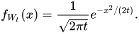
Brownian motion is a centered Gaussian process. In particular, for $t>0$ , $W_{t}=W_{t}-W_{0}\sim N(0,t)$ , that is, the probability density function of $W_{t}$ is

$f_{W_{t}}(x)={\frac {1}{\sqrt {2\pi t}}}e^{-x^{2}/(2t)}.$

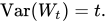
The covariance between $W_{t}$ and $W_{s}$ ( ${\textstyle s\leq t$ ) is $\operatorname {cov} (W_{s},W_{t})=\operatorname {E} [W_{s}W_{t}]=s.$ In particular, the variance is $\operatorname {Var} (W_{t})=t.$

The correlation between $W_{t}$ and $W_{s}$ ( ${\textstyle s\leq t$ ) is

$\operatorname {corr} (W_{s},W_{t})={\frac {\operatorname {cov} (W_{s},W_{t})}{\sigma _{W_{s}}\sigma _{W_{t}}}}={\frac {s}{\sqrt {st}}}={\sqrt {\frac {s}{t}}}.$

A useful decomposition for proving martingale properties, also called Brownian increment decomposition, is

$W_{t}=W_{s}+(W_{t}-W_{s}),\;s\leq t.$

Brownian motion is a Lévy process. In particular, it has stationary and independent increments.
Brownian motion is a continuous martingale.
Brownian motion has the strong Markov property.

Covariance and correlation

The covariance and correlation between $W_{t}$ and $W_{s}$ follow from the definition that non-overlapping increments are independent, of which only the property that they are uncorrelated is used. Suppose that ${\textstyle t_{1}\leq t_{2}$ .

$\operatorname {cov} (W_{t_{1}},W_{t_{2}})=\operatorname {E} \left[(W_{t_{1}}-\operatorname {E} [W_{t_{1}}])\cdot (W_{t_{2}}-\operatorname {E} [W_{t_{2}}])\right]=\operatorname {E} \left[W_{t_{1}}\cdot W_{t_{2}}\right].$

Substituting $W_{t_{2}}=(W_{t_{2}}-W_{t_{1}})+W_{t_{1}}$ we arrive at: ${\begin{aligned}\operatorname {E} [W_{t_{1}}\cdot W_{t_{2}}]&=\operatorname {E} \left[W_{t_{1}}\cdot ((W_{t_{2}}-W_{t_{1}})+W_{t_{1}})\right]\\&=\operatorname {E} \left[W_{t_{1}}\cdot (W_{t_{2}}-W_{t_{1}})\right]+\operatorname {E} \left[W_{t_{1}}^{2}\right].\end{aligned}}$

Since ${\textstyle W_{t_{1}}=W_{t_{1}}-W_{t_{0}}$ and ${\textstyle W_{t_{2}}-W_{t_{1}}$ are independent, $\operatorname {E} \left[W_{t_{1}}\cdot (W_{t_{2}}-W_{t_{1}})\right]=\operatorname {E} [W_{t_{1}}]\cdot \operatorname {E} [W_{t_{2}}-W_{t_{1}}]=0.$

Thus $\operatorname {cov} (W_{t_{1}},W_{t_{2}})=\operatorname {E} \left[W_{t_{1}}^{2}\right]=t_{1}.$

A corollary useful for simulation is that we can write, for t₁ < t₂: $W_{t_{2}}=W_{t_{1}}+{\sqrt {t_{2}-t_{1}}}\cdot Z$ where Z is an independent standard normal variable.

Infinitesimal generator

The infinitesimal generator of Brownian motion is given by

$Af(x)=\lim _{t\to 0}{\frac {\operatorname {E} [f(W_{t}+x)]-f(x)}{t}}={\frac {1}{2}}f''(x),\quad x\in \mathbb {R} ,$

for all $f\in C^{2}(\mathbb {R} )$ that vanish at infinity. This is an almost direct consequence of Itô's formula.

Running maximum

The joint distribution of the running maximum

$M_{t}=\max _{0\leq s\leq t}W_{s}$

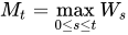
and W_t is

$f_{M_{t},W_{t}}(m,w)={\frac {2(2m-w)}{t{\sqrt {2\pi t}}}}e^{-{\frac {(2m-w)^{2}}{2t}}},\qquad m\geq 0,w\leq m.$

To get the unconditional distribution of ${\textstyle f_{M_{t}}$ , integrate over −∞ < w ≤ m: ${\begin{aligned}f_{M_{t}}(m)&=\int _{-\infty }^{m}f_{M_{t},W_{t}}(m,w)\,dw=\int _{-\infty }^{m}{\frac {2(2m-w)}{t{\sqrt {2\pi t}}}}e^{-{\frac {(2m-w)^{2}}{2t}}}\,dw\\[5pt]&={\sqrt {\frac {2}{\pi t}}}e^{-{\frac {m^{2}}{2t}}},\qquad m\geq 0,\end{aligned}}$

the probability density function of a Half-normal distribution. The expectation is $\operatorname {E} [M_{t}]=\int _{0}^{\infty }mf_{M_{t}}(m)\,dm=\int _{0}^{\infty }m{\sqrt {\frac {2}{\pi t}}}e^{-{\frac {m^{2}}{2t}}}\,dm={\sqrt {\frac {2t}{\pi }}}$

If at time t the Wiener process has a known value ${\textstyle W_{t}$ , it is possible to calculate the conditional probability distribution of the maximum in interval ${\textstyle [0,t]$ (cf. Probability distribution of extreme points of a Wiener stochastic process). The cumulative probability distribution function of the maximum value, conditioned by the known value ${\textstyle W_{t}$ , is: $\,F_{M_{W_{t}}}(m)=\Pr \left(M_{W_{t}}=\max _{0\leq s\leq t}W_{s}\leq m\mid W_{t}\right)=\ 1-\ e^{-2{\frac {m(m-W_{t})}{t}}}\ \,,\,\ \ m>\max(0,W_{t})$

Arcsine laws

There are multiple (random) quantities $T$ related to Brownian motion that follow the arcsine distribution:

$\Pr(T\leq t)={\frac {2}{\pi }}\arcsin({\sqrt {t}}),\quad t\in [0,1].$

These statements are referred to as the arcsine laws of Brownian motion.

First arcsine law

The amount of time Brownian motion is positive, that is,

$T=\int _{0}^{1}1_{\{W_{t}>0\}}\mathrm {d} t,$

is arcsine-distributed.

Second arcsine law

The last time Brownian motion hits zero in the time interval $[0,1]$ , that is,

$T=\sup\{t\leq 1:W_{t}=0\},$

is arcsine-distributed.

Third arcsine law

The time at which Brownian motion attains its maximum on $[0,1]$ , that is,

$T=\inf \left\{t\leq 1:W_{t}=\max _{s\in [0,1]}W_{s}\right\},$

is arcsine-distributed.

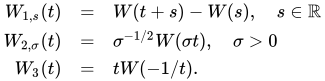
Self-similarity

Brownian scaling

For every c > 0 the process ${\textstyle V_{t}=(1/{\sqrt {c}})W_{ct}$ is another Wiener process.

Time reversal

The process ${\textstyle V_{t}=W_{1-t}-W_{1}$ for 0 ≤ t ≤ 1 is distributed like W_t for 0 ≤ t ≤ 1.

Time inversion

The process ${\textstyle V_{t}=tW_{1/t}$ is another Wiener process.

Projective invariance

Consider a Wiener process ${\textstyle W(t)$ , ${\textstyle t\in \mathbb {R}$ , conditioned so that ${\textstyle \lim _{t\to \pm \infty }tW(t)=0$ (which holds almost surely) and as usual ${\textstyle W(0)=0$ . Then the following are all Wiener processes: ${\begin{array}{rcl}W_{1,s}(t)&=&W(t+s)-W(s),\quad s\in \mathbb {R} \\W_{2,\sigma }(t)&=&\sigma ^{-1/2}W(\sigma t),\quad \sigma >0\\W_{3}(t)&=&tW(-1/t).\end{array}}$ Thus the Wiener process is invariant under the projective group PSL(2,R), being invariant under the generators of the group. The action of an element ${\textstyle g={\begin{bmatrix}a&b\\c&d\end{bmatrix}}$ is $W_{g}(t)=(ct+d)W\left({\frac {at+b}{ct+d}}\right)-ctW\left({\frac {a}{c}}\right)-dW\left({\frac {b}{d}}\right),$ which defines a group action, in the sense that ${\textstyle (W_{g})_{h}=W_{gh}.$

Conformal invariance in two dimensions

Let ${\textstyle W$ be a two-dimensional Wiener process, regarded as a complex-valued process with ${\textstyle W_{0}=0\in \mathbb {C}$ . Let ${\textstyle D\subset \mathbb {C}$ be an open set containing 0, and ${\textstyle \tau _{D}$ be associated Markov time: $\tau _{D}=\inf\{t\geq 0|W_{t}\not \in D\}.$ If ${\textstyle f:D\to \mathbb {C}$ is a holomorphic function which is not constant, such that ${\textstyle f(0)=0$ , then ${\textstyle f(W_{t})$ is a time-changed Wiener process in ${\textstyle f(D)$ . More precisely, the process ${\textstyle Y$ is Wiener in D with the Markov time ${\textstyle S$ , where $Y_{t}=f(W_{\sigma (t)})$ $S(t)=\int _{0}^{t}|f'(W_{s})|^{2}\,ds$ $\sigma (t)=S^{-1}(t):\quad t=\int _{0}^{\sigma (t)}|f'(W_{s})|^{2}\,ds.$

Stopping times

Hitting time of level sets

The first hitting time $T_{a}$ of the Wiener process of some value $a>0$ , that is,

$T_{a}=\inf\{t\geq 0:W_{t}=a\},$

is Lévy-distributed, which means it has the Lebesgue density

$f(t)={\frac {a}{\sqrt {2\pi t^{3}}}}\exp \left(-{\frac {a^{2}}{2t}}\right)1_{[0,\infty )}(t),\quad t\in \mathbb {R} .$

In particular, $\operatorname {E} [T_{a}]=\infty$ . Moreover, $T_{a}$ has the same distribution as $a^{2}/W_{1}^{2}$ .

Exit time of intervals

Let $\tau _{a}$ be the first exit time of the interval $[-a,a]$ . Its expectation equals

$\operatorname {E} [\tau _{a}]=a^{2},$

and its Laplace transform is

$\operatorname {E} [e^{-t\tau _{a}}]={\frac {1}{\cosh(a{\sqrt {2t}})}},\quad t\geq 0.$

Hitting times of two level sets

Let $a<0<b$ and $T_{c}=\inf\{t\geq 0:W_{t}=c\}$ be the first hitting time of a value $c\in \mathbb {R}$ . Then,

$\operatorname {P} (T_{a}<T_{b})={\frac {b}{b-a}},\qquad \operatorname {P} (T_{b}<T_{a})=-{\frac {a}{b-a}}.$

A class of Brownian martingales

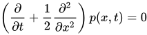
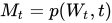
If a polynomial p(x, t) satisfies the partial differential equation $\left({\frac {\partial }{\partial t}}+{\frac {1}{2}}{\frac {\partial ^{2}}{\partial x^{2}}}\right)p(x,t)=0$ then the stochastic process $M_{t}=p(W_{t},t)$ is a martingale.

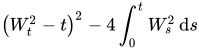
Example: ${\textstyle W_{t}^{2}-t$ is a martingale, which shows that the quadratic variation of W on [0, t] is equal to t. It follows that the expected time of first exit of W from (−c, c) is equal to c².

More generally, for every polynomial p(x, t) the following stochastic process is a martingale: $M_{t}=p(W_{t},t)-\int _{0}^{t}a(W_{s},s)\,\mathrm {d} s,$ where a is the polynomial $a(x,t)=\left({\frac {\partial }{\partial t}}+{\frac {1}{2}}{\frac {\partial ^{2}}{\partial x^{2}}}\right)p(x,t).$

Example: ${\textstyle p(x,t)=\left(x^{2}-t\right)^{2},$ ${\textstyle a(x,t)=4x^{2};$ the process $\left(W_{t}^{2}-t\right)^{2}-4\int _{0}^{t}W_{s}^{2}\,\mathrm {d} s$ is a martingale, which shows that the quadratic variation of the martingale ${\textstyle W_{t}^{2}-t$ on [0, t] is equal to $4\int _{0}^{t}W_{s}^{2}\,\mathrm {d} s.$

About functions p(xa, t) more general than polynomials, see local martingales.

Properties of sample paths

The set of all functions w with the following properties has probability one under the Wiener measure. That is, a path (sample function) of the Wiener process has all these properties almost surely:

Qualitative properties

For every ε > 0, the function w takes both (strictly) positive and (strictly) negative values on (0, ε).
The function w is continuous everywhere, but nowhere differentiable (like the Weierstrass function).
For any ${\textstyle \epsilon >0$ , ${\textstyle w$ is nowhere ${\textstyle ({\tfrac {1}{2}}+\epsilon )$ -Hölder continuous, but it is locally ${\textstyle ({\tfrac {1}{2}}-\epsilon )$ -Hölder continuous.
Points of local maximum of the function w are a dense countable set; the maximum values are pairwise different; each local maximum is sharp in the following sense: if w has a local maximum at t then $\lim _{s\to t}{\frac {|w(s)-w(t)|}{|s-t|}}=\infty .$ The same holds for local minima.
The function w has no points of local increase, that is, no t > 0 satisfies the following for some ε in (0, t): first, w(s) ≤ w(t) for all s in (t − ε, t), and second, w(s) ≥ w(t) for all s in (t, t + ε). (Local increase is a weaker condition than that w is increasing on (t − ε, t + ε).) The same holds for local decrease.
The function w is of unbounded variation on every interval.
The quadratic variation of w over [0,t] is t.
The set $\{t\geq 0:w(t)=0\}$ of Zeros of the function w is perfect (closed and contains no isolated points), is nowhere dense, has Lebesgue measure 0 and has Hausdorff dimension 1/2 (therefore, is uncountable).

While it is not true that a path of Brownian motion is almost surely nowhere ${\textstyle {\tfrac {1}{2}}$ -Hölder continuous, for a fixed $t\geq 0$ , it can be asserted that a path is almost surely not ${\textstyle {\tfrac {1}{2}}$ -Hölder continuous in $t$ .

Quantitative properties

Law of the iterated logarithm

$\limsup _{t\to +\infty }{\frac {|w(t)|}{\sqrt {2t\log \log t}}}=1,\quad {\text{almost surely}}.$

Modulus of continuity

Local modulus of continuity: $\limsup _{\varepsilon \to 0+}{\frac {|w(\varepsilon )|}{\sqrt {2\varepsilon \log \log(1/\varepsilon )}}}=1,\qquad {\text{almost surely}}.$

Global modulus of continuity (Lévy): $\limsup _{\varepsilon \to 0+}\sup _{0\leq s<t\leq 1,t-s\leq \varepsilon }{\frac {|w(s)-w(t)|}{\sqrt {2\varepsilon \log(1/\varepsilon )}}}=1,\qquad {\text{almost surely}}.$

Dimension doubling theorem

The dimension doubling theorems say that the Hausdorff dimension of a set under a Brownian motion doubles almost surely.

Local time

The image of the Lebesgue measure on [0, t] under the map w (the pushforward measure) has a density L_t. Thus, $\int _{0}^{t}f(w(s))\,\mathrm {d} s=\int _{-\infty }^{+\infty }f(x)L_{t}(x)\,\mathrm {d} x$ for a wide class of functions f (namely: all continuous functions; all locally integrable functions; all non-negative measurable functions). The density L_t is (more exactly, can and will be chosen to be) continuous. The number L_t(x) is called the local time at x of w on [0, t]. It is strictly positive for all x of the interval (a, b) where a and b are the least and the greatest value of w on [0, t], respectively. (For x outside this interval the local time evidently vanishes.) Treated as a function of two variables x and t, the local time is still continuous. Treated as a function of t (while x is fixed), the local time is a singular function corresponding to a nonatomic measure on the set of zeros of w.

These continuity properties are fairly non-trivial. Consider that the local time can also be defined (as the density of the pushforward measure) for a smooth function. Then, however, the density is discontinuous, unless the given function is monotone. In other words, there is a conflict between good behavior of a function and good behavior of its local time. In this sense, the continuity of the local time of the Wiener process is another manifestation of non-smoothness of the trajectory.

Information rate

The information rate of the Wiener process with respect to the squared error distance, i.e. its quadratic rate-distortion function, is given by $R(D)={\frac {2}{\pi ^{2}D\ln 2}}\approx 0.29D^{-1}.$ Therefore, it is impossible to encode ${\textstyle \{w_{t}\}_{t\in [0,T]}$ using a binary code of less than ${\textstyle TR(D)$ bits and recover it with expected mean squared error less than D. On the other hand, for any ${\textstyle \varepsilon >0$ , there exists T large enough and a binary code of no more than ${\textstyle 2^{TR(D)}$ distinct elements such that the expected mean squared error in recovering ${\textstyle \{w_{t}\}_{t\in [0,T]}$ from this code is at most ${\textstyle D-\varepsilon$ .

In many cases, it is impossible to encode the Wiener process without sampling it first. When the Wiener process is sampled at intervals ${\textstyle T_{s}$ before applying a binary code to represent these samples, the optimal trade-off between code rate ${\textstyle R(T_{s},D)$ and expected mean square error D (in estimating the continuous-time Wiener process) follows the parametric representation $R(T_{s},D_{\theta })={\frac {T_{s}}{2}}\int _{0}^{1}\log _{2}^{+}\left[{\frac {S(\varphi )-{\frac {1}{6}}}{\theta }}\right]d\varphi ,$ $D_{\theta }={\frac {T_{s}}{6}}+T_{s}\int _{0}^{1}\min \left\{S(\varphi )-{\frac {1}{6}},\theta \right\}d\varphi ,$ where ${\textstyle S(\varphi )=(2\sin(\pi \varphi /2))^{-2}$ and ${\textstyle \log ^{+}[x]=\max\{0,\log(x)\}$ . In particular, ${\textstyle T_{s}/6$ is the mean squared error associated only with the sampling operation (without encoding).

A single realization of a three-dimensional Wiener process

03d-dimensional Wiener process

A Wiener process can be straighforwardly extended to higher dimensions $d\geq 2$ as follows.

Definition

A process $W=(W^{1},\dots ,W^{d})$ is a $d$ -dimensional Wiener process, if $W^{1},\dots ,W^{d}$ are independent one-dimensional Wiener processes.

Lévy characterization

Let $W=(W^{1},\dots ,W^{d})$ be an adapted stochastic process. The following are equivalent:

$W$ is a $d$ -dimensional Wiener process.
$W^{1},\dots ,W^{d}$ are continuous local martingales and for $i,j\in \{1,\dots ,d\}$ , the covariation fulfills $\langle W^{i},W^{j}\rangle _{t}=\delta _{ij}t$ for all $t\geq 0$ , where $\delta _{ij}$ is the Kronecker delta.

Generator representation

The Wiener process can also be defined as the unique continuous Markov process starting in zero almost surely and whose generator is $A={\frac {1}{2}}\Delta$ with domain $\mathrm {Dom} (A)=\{f\in C^{2}(\mathbb {R} ^{d}):f,\partial _{ij}^{2}f\in C_{0}(\mathbb {R} ^{d})\}$ , where $C_{0}(\mathbb {R} ^{d})$ denotes the space of continuous functions vanishing at infinity.

In fact, given the above generator $A$ , there exist a unique Feller semigroup $(P_{t})_{t\geq 0}$ , that is, $P_{t}$ is a Markov kernel with

$\forall x\in \mathbb {R} ^{d}:P_{0}(x,\cdot )=\delta _{x}$ , the Dirac measure,
$\forall s,t\geq 0,\,A\in {\mathcal {B}}(\mathbb {R} ^{d}):P_{t+s}(x,A)=\int _{\mathbb {R} ^{d}}P_{t}(y,A)P_{s}(x,\mathrm {d} y)$ ,
$\forall f\in C_{0}(\mathbb {R} ^{d}):P_{t}f\equiv \int _{\mathbb {R} ^{d}}f(y)P_{t}(\cdot ,\mathrm {d} y)\in C_{0}(\mathbb {R} ^{d})$ ,
$\forall f\in C_{0}(\mathbb {R} ^{d}):\lim _{t\to 0}\lVert P_{t}f-f\rVert _{L^{\infty }(\mathbb {R} ^{d})}=0$ .

such that

$Af=\lim _{t\to 0}{\frac {P_{t}f-f}{t}},\qquad f\in \mathrm {Dom} (A).$

In this case, for $f\in \mathrm {Dom} (A)$ , the correspondence is precisely

$P_{t}f(x)=e^{At}f(x)=\int _{\mathbb {R} ^{d}}{\frac {1}{(2\pi t)^{d/2}}}\exp \left(-{\frac {\lVert x-y\rVert ^{2}}{2t}}\right)f(y)\mathrm {d} y,\quad x\in \mathbb {R} ^{d}.$

At the same time, there exist a unique Markov process $W$ on $(\mathbb {R} ^{[0,\infty )},{\mathcal {B}}(\mathbb {R} )^{\otimes [0,\infty )})$ starting in zero such that

$\mathrm {Pr} (W_{t}+x\in \cdot )=P_{t}(x,\cdot ),\qquad \forall t\geq 0,\,x\in \mathbb {R} ^{d},$

that is, the transition probabilities of $W_{t}+x$ are given by $P_{t}(x,\cdot )$ . Finally, by Kolmorov's continuity criterion, there exists a modification of $W$ with continuous paths, which is the Wiener process.

Five sampled processes, with expected standard deviation in gray

04Properties of a d-dimensional Wiener process

Path properties

The following path properties hold almost surely (some of them follow directly from those of the one-dimensional Wiener process):

The paths are everywhere continuous, but nowhere differentiable.
For any ${\textstyle \epsilon >0$ , the paths are nowhere ${\textstyle ({\tfrac {1}{2}}+\epsilon )$ -Hölder continuous, but locally ${\textstyle ({\tfrac {1}{2}}-\epsilon )$ -Hölder continuous.
For $d=2$ , the Wiener process is recurrent, that is, for every Borel set $A$ , if the first hitting time $\inf\{t>0:W_{t}\in A\}$ is not almost surely infinite, then $\operatorname {Pr} (W_{t}\in A{\text{ for infinitely many }}t>0)=1$ . In particular, the Wiener process returns arbitrarily close to the origin infinitely often almost surely.
For $d\geq 3$ , every compact set $K$ is transient, that is, the last hitting time $\sup\{t\geq 0:W_{t}\in K\}$ is almost surely finite. In particular, the Wiener process returns in a neighborhood of the origin only finitely many times almost surely.

Infinitesimal generator

Similarly to the one-dimensional case, the infinitesimal generator of Brownian motion is given by

$Af(x)=\lim _{t\to 0}{\frac {\operatorname {E} [f(W_{t}+x)]-f(x)}{t}}={\frac {1}{2}}\Delta f(x),\quad x\in \mathbb {R} ^{d},$

where $\Delta$ is the Laplace operator, for all $f\in C^{2}(\mathbb {R} ^{d})$ that vanish at infinity.

Harmonic measure on the sphere

The harmonic measure of Brownian motion on the sphere $\mathbb {S} _{d-1}$ , that is, the distribution of $W_{\tau }$ , where $\tau =\inf\{t\geq 0:W_{t}\in \mathbb {S} _{d-1}\}$ is the first hitting time of the unit sphere, when the process is started in $x\in B_{1}(0)$ , is

$\mu ^{x}(A)\equiv \operatorname {Pr} (W_{\tau }+x\in A)=\int _{\mathbb {S} _{d-1}}1_{A}(y)q(x,y)\mathrm {d} \sigma (y),\qquad A\in {\mathcal {B}}(\mathbb {R} ^{d}),$

where $\sigma$ is the surface measure and

$q(x,y)={\frac {1}{\sigma (\mathbb {S} _{d-1})}}{\frac {1-\lVert x\rVert ^{2}}{\lVert x-y\rVert ^{d}}},\quad x\in B_{1}(0),\,y\in \mathbb {S} _{d-1},$

is the Poisson kernel for the unit ball.

Occupation time formula

Let $D\subset \mathbb {R} ^{d}$ be an open, bounded set and $\tau _{D}^{x}=\inf\{t\geq 0:W_{t}+x\in \partial D\}$ be the first exit time of Brownian motion, when started in $x\in D$ . Then, the occupation time of a set $A\in {\mathcal {B}}(\mathbb {R} ^{d})$ is given by

$\operatorname {E} \left[\int _{0}^{\tau _{D}^{x}}1_{A}(W_{t}+x)\mathrm {d} t\right]=\int _{\mathbb {R} ^{d}}1_{A}(y)G(x,y)\mathrm {d} y,$

where $G$ is the Green function of the Laplace operator for the domain $D$ , that is, the (distributional) solution of the equation

${\begin{aligned}-\Delta G(x,\cdot )&=\delta _{x},\quad \ \ \,{\text{in }}D\\G(x,\cdot )&=0,\qquad {\text{on }}\partial D\end{aligned}}$

where $\delta _{x}$ is the Dirac measure in $x$ . More generally, for a measurable function $f$ that is either non-negative or integrable with respect to $G(x,\cdot )\mathrm {d} \lambda$ , it holds

$\operatorname {E} \left[\int _{0}^{\tau _{D}^{x}}f(W_{t}+x)\mathrm {d} t\right]=\int _{\mathbb {R} ^{d}}f(y)G(x,y)\mathrm {d} y.$

Representation of harmonic functions

Let $D\subset \mathbb {R} ^{d}$ be a bounded open set. Let $u$ be harmonic ( $\Delta u=0$ ) in $D$ and continuous in ${\bar {D}}$ . Then,

$u(x)=\operatorname {E} [u(W_{\tau _{D}^{x}}+x)],\quad x\in {\bar {D}},$

where $\tau _{D}^{x}=\inf\{t\geq 0:W_{t}+x\in D^{c}\}$ is the first exit time of the Wiener process from $D$ when started in $x$ .

Stopping times

Moments of exit times

Let $D\subset \mathbb {R} ^{d}$ be a bounded open domain with smooth boundary and let $\tau _{x}=\inf\{t\geq 0:W_{t}+x\in D^{c}\}$ . Then, for $k\in \mathbb {N}$ , the function

$u_{k}(x)=\operatorname {E} [\tau _{x}^{k}],\quad x\in {\bar {D}},$

is the solution to the recursive differential equation

${\begin{cases}&{\frac {1}{2}}\Delta u_{1}+1=0,&k=1\\&{\frac {1}{2}}\Delta u_{k}+ku_{k-1}=0,&k\geq 2\end{cases}}\quad {\text{ on }}D$

with the boundary condition $u_{k}=0$ on $\partial D$ . In particular, when $D$ is the ball with radius $R$ , then

$\operatorname {E} [\tau _{x}]={\frac {R^{2}-\lVert x\rVert ^{2}}{d}}.$

Distribution of exit time from a ball

Let $\tau _{R}=\inf\{t\geq 0:W_{t}\notin B_{R}\}$ be the first exit time of Brownian motion from the ball with radius $R$ and centered in the origin. Then

$\operatorname {Pr} (\tau _{R}>t)=\sum _{k=1}^{\infty }c_{k,d}\exp \left(-{\frac {q_{k,d}^{2}}{2R^{2}}}t\right),$

where $q_{1,d}<q_{2,d}<\dots$ are the positive roots of the Bessel function $J_{d/2-1}$ and

$c_{k,d}={\frac {q_{k,d}^{d/2-2}}{2^{d/2-2}\Gamma (d/2)J_{d/2}(q_{k,d})}}$

with the Gamma function $\Gamma$ . In particular, $\tau _{R}$ has exponential tails.

A demonstration of Brownian scaling, showing for decreasing c. Note that the average features of the function do not change while zooming in, and note that it zooms in quadratically faster horizontally than vertically.

05Wiener process on Riemannian manifolds

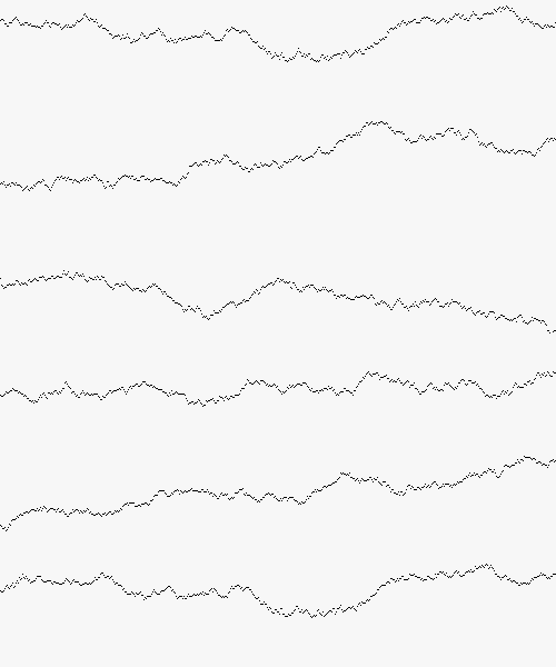
The Wiener process can be generalized in such a way that it evolves only on a Riemannian manifold $M\subset \mathbb {R} ^{d}$ such as a sphere. This requires the orthogonal projections $P(x)$ onto the tangent space $T_{x}M$ for all $x\in M$ . With this definition, the Wiener process $X$ on $M$ is defined as the solution to the Stratonovich equation $\mathrm {d} X_{t}^{i}=\sum _{j=1}^{d}P(x)_{ij}\circ \mathrm {d} W_{t}^{j},\qquad X_{0}\in M,$ where $W=(W^{1},\dots ,W^{d})$ is a $d$ -dimensional standard Wiener process. It can be shown that $X$ indeed evolves in $M$ (which would not be case the solution to the same equation with the Stratonovich replaced by the Itô integral). Moreover, the infinitesimal generator of $X$ is one-half the Laplace-Beltrami operator, which is a generalization of the Laplace operator for Riemannian manifolds.

The special case of the unit sphere $\mathbb {S} _{d-1}$ possesses the projection operator $P(x)y=y-\langle y,x\rangle x,\quad y\in \mathbb {R} ^{d},$ which leads to the Stroock representation of spherical Brownian motion $X_{t}=X_{0}+\int _{0}^{t}(\delta _{ij}-X_{s}^{i}X_{s}^{j})\circ \mathrm {d} W_{s}^{j}.$

The generator of Brownian motion on Riemannian manifolds is 1⁄2 times the Laplace-Beltrami operator. The image above shows Brownian motion on the surface of a 2-sphere.

06Infinite dimensional Wiener process

The Wiener process can be generalized to a process taking values in an arbitrary separable Hilbert space (which means it possesses an orthonormal basis), although some technical difficulties arise. The construction of a Hilbert space-valued Wiener process is the starting point for stochastic partial differential equations, which are generalizations of partial differential equations driven by a Wiener process in time.

The definition of the Wiener process on a separable Hilbert space $(H,\langle \cdot ,\cdot \rangle )$ requires the notion of a Gaussian random variable on $H$ . Similarly to the $d$ -dimensional case with $d>1$ , a random variable $Z$ with values in $(H,{\mathcal {B}}(H))$ is Gaussian if for all $h\in H$ the projection $\langle Z,h\rangle$ is univariate Gaussian. One can show that the law of $Z$ is uniquely determined by its mean $m\in H$ and covariance operator $Q$ (non-negative, symmetric and the series of eigenvalues is summable) via

${\begin{aligned}&\operatorname {E} [\langle Z,h\rangle ]=\langle m,h\rangle ,\\&\operatorname {E} [\langle Z-m,g\rangle \langle Z-m,h\rangle ]=\langle g,Qh\rangle .\end{aligned}}$

In this case, one writes $Z\sim {\mathcal {N}}(m,Q)$ .

The condition that the eigenvalues $(\lambda _{k})_{k\in \mathbb {N} }$ of $Q$ fulfill

$\sum _{k=1}^{\infty }|\lambda _{k}|<\infty$

is called trace-class and excludes, in particular, the identity operator from the definition.

Q-Wiener process

Given a non-negative, symmetric, trace-class operator $Q$ , a stochastic process $W^{Q}=(W_{t}^{Q})_{t\geq 0}$ with values in $H$ is a $Q$ -Wiener process if

$W_{0}^{Q}=0$ ,
$W^{Q}$ has continuous trajectories, i.e., for all $\omega \in \Omega$ and $t\geq 0$

$\lim _{s\to t}\lVert W_{s}(\omega )-W_{t}(\omega )\rVert =0$ ,

$W^{Q}$ has independent increments, i.e., for all $0\leq t_{1}<\dots <t_{n}$ and $n\in \mathbb {N}$

$W_{t_{1}}^{Q},\,W_{t_{2}}^{Q}-W_{t_{1}}^{Q},\dots ,\,W_{t_{n}}^{Q}-W_{t_{n-1}}^{Q}$ are independent,

the increments are centered Gaussian, namely $W_{t}^{Q}-W_{s}^{Q}\sim {\mathcal {N}}{\big (}0,(t-s)Q{\big )}$ for $s<t$ .

Equivalently, the process can be defined as a series expansion of independent one-dimensional Wiener processes $(\beta _{k})_{k\in \mathbb {N} }$ in the basis $(e_{k})_{k\in \mathbb {N} }$ of eigenvectors of $Q$ via

$W_{t}^{Q}=\sum _{k=1}^{\infty }{\sqrt {\lambda }}_{k}\beta _{k}(t)e_{k}.$

This justifies the need to require $Q$ to be trace-class, since

$\operatorname {E} {\big [}\lVert W_{t}^{Q}\rVert ^{2}{\big ]}=t\sum _{k=1}^{\infty }|\lambda _{k}|,$

which would otherwise diverge.

Cylindrical Wiener process

The fact that one cannot define a Wiener process on $H$ with covariance operator $Q=I$ (the identity) is unsatisfying. Thus, another approach is required to make sense of

$W_{t}=\sum _{k=1}^{\infty }\beta _{k}(t)e_{k},$

for independent one-dimensional Wiener processes $(\beta _{k})_{k\in \mathbb {N} }$ and an orthonormal basis $(e_{k})_{k\in \mathbb {N} }$ of $H$ . One possibility consists in evaluating the process only in specific "directions" $h\in H$ in space. For a $Q$ -Wiener process $W^{Q}$ with a trace class operator $Q$ (which is a well-defined process on $H$ ), the projection onto the direction $h$ is

$_{h}W_{t}^{Q}:=\langle W_{t}^{Q},h\rangle .$

The family $(_{h}W^{Q})_{h\in H}$ is a collection of one-dimensional continuous Gaussian processes with

${\begin{aligned}&\operatorname {E} [_{h}W_{t}^{Q}]=0,\qquad &&\forall h\in H\\&\operatorname {E} [_{h}W_{t}^{Q}\,_{g}W_{s}^{Q}]=(t\land s)\langle h,Qg\rangle ,\qquad &&\forall h,g\in H.\end{aligned}}$

The above equations still uniquely characterise the process $W^{Q}$ , but it does not require that $Q$ must be trace class anymore. Thus, going all the way back, a collection $(_{h}W)_{h\in H}$ of one-dimensional continuous Gaussian processes is called a cylindrical Wiener process if

${\begin{aligned}&\operatorname {E} [_{h}W_{t}]=0,&&\forall h\in H,\\&\operatorname {E} [_{h}W_{t}\,_{g}W_{s}]=(t\land s)\langle h,g\rangle ,&&\forall h,g\in H.\end{aligned}}$

This definition does not define a process $W$ on $H$ with covariance operator $Q=I$ , but the processes $_{h}W$ behave as if they were the projections $\langle W,h\rangle$ of the process $W$ if it would exist.

It is also possible to define $W$ by embedding it linearly into another Hilbert space $(H_{1},\langle \cdot ,\cdot \rangle _{1})$ , in which the series representation does converge. This can be realised, for example, by taking $H_{1}=H$ , the embedding $J:(H,\langle \cdot ,\cdot \rangle )\to (H,\langle \cdot ,\cdot \rangle _{1})$ being the identity and

$\langle h,g\rangle _{1}:=\sum _{k=1}^{\infty }{\frac {1}{k^{2}}}\langle h,e_{k}\rangle \langle g,e_{k}\rangle ,\quad h,g\in H,$

for an orthonormal basis $(e_{k})_{k\in \mathbb {N} }$ of $H$ with respect to $\langle \cdot ,\cdot \rangle$ . In this case,

${\tilde {W}}_{t}:=\sum _{k=1}^{\infty }\beta _{k}(t)J(e_{k})$

is a well-defined $I$ -Wiener process on $H_{1}$ , since

$\sum _{k=1}^{\infty }\langle e_{k},Ie_{k}\rangle _{1}=\sum _{k=1}^{\infty }{\frac {1}{k^{2}}}<\infty ,$

and it is also called a cylindrical Wiener process on $H$ . Many other pairs of surrogate Hilbert space $(H_{1},\langle \cdot ,\cdot \rangle _{1})$ and embedding $J$ are possible for this construction.

Once again, ${\tilde {W}}$ is not a process on $(H,\langle \cdot ,\cdot \rangle )$ but on $(H_{1},\langle \cdot ,\cdot \rangle _{1})$ , which is either not the space or not the inner product one is interested in. The surrogate Hilbert space $(H_{1},\langle \cdot ,\cdot \rangle _{1})$ is merely used as a ground on which ${\tilde {W}}$ can be reasonably defined, but due to the injectivity of $J$ , one may think of ${\tilde {W}}$ as the unique representative of $W$ on the space $(H_{1},\langle \cdot ,\cdot \rangle _{1})$ .

Wiener processes with drift (blue) and without drift (red)

07Related processes

Wiener process with drift

The stochastic process defined by $X_{t}=\mu t+\sigma W_{t}$ for $\mu \in \mathbb {R}$ is called a Wiener process with drift μ and infinitesimal variance σ²>0. These processes exhaust continuous Lévy processes, which means that they are the only continuous Lévy processes, as a consequence of the Lévy-Khintchine representation.

Brownian bridge

Two random processes on the time interval [0, 1] appear, roughly speaking, when conditioning the Wiener process to vanish on both ends of [0,1]. With no further conditioning, the process takes both positive and negative values on [0, 1] and is called Brownian bridge. Conditioned also to stay positive on (0, 1), the process is called Brownian excursion. In both cases a rigorous treatment involves a limiting procedure, since the formula P(A|B) = P(A ∩ B)/P(B) does not apply when P(B) = 0.

Geometric Brownian motion

The geometric Brownian motion is defined as

$S_{t}=e^{\mu t-{\frac {\sigma ^{2}t}{2}}+\sigma W_{t}}.$

It is a stochastic process which is used to model processes that can never take on negative values, such as the value of stocks.

Ornstein-Uhlenbeck process

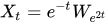
The stochastic process $X_{t}=e^{-t}W_{e^{2t}}$ is distributed like the Ornstein-Uhlenbeck process with parameters ${\textstyle \theta =1$ , ${\textstyle \mu =0$ , and ${\textstyle \sigma ^{2}=2$ .

Integrated Brownian motion

The time-integral of the Wiener process $W_{t}^{(-1)}:=\int _{0}^{t}W_{s}\,ds$ is called integrated Brownian motion or integrated Wiener process. It arises in many applications and can be shown to have the distribution N(0, t³/3) using Fubini's theorem and the fact that the covariance of the Wiener process is ${\textstyle t\wedge s=\min(t,s)$ .

A more general process can be defined by $V_{f}(t)=\int _{0}^{t}f'(s)W_{s}\,ds=\int _{0}^{t}(f(t)-f(s))\,dW_{s}.$ Then, for ${\textstyle a>0$ , $\operatorname {Var} (V_{f}(t))=\int _{0}^{t}(f(t)-f(s))^{2}\,ds,$ $\operatorname {cov} (V_{f}(t+a),V_{f}(t))=\int _{0}^{t}(f(t+a)-f(s))(f(t)-f(s))\,ds.$ In fact, ${\textstyle V_{f}(t)$ is always a zero mean normal random variable. This allows for simulation of ${\textstyle V_{f}(t+a)$ given ${\textstyle V_{f}(t)$ by taking $V_{f}(t+a)=A\cdot V_{f}(t)+B\cdot Z$ where Z is a standard normal variable and $A={\frac {\operatorname {cov} (V_{f}(t+a),V_{f}(t))}{\operatorname {Var} (V_{f}(t))}},$ $B^{2}=\operatorname {Var} (V_{f}(t+a))-A^{2}\operatorname {Var} (V_{f}(t)).$ The case of ${\textstyle V_{f}(t)=W_{t}^{(-1)}$ corresponds to ${\textstyle f(t)=t$ . All these results can be seen as direct consequences of the Itô isometry. The n-times-integrated Wiener process is a zero-mean normal variable with variance ${\textstyle {\frac {t}{2n+1}}\left({\frac {t^{n}}{n!}}\right)^{2}$ . This is given by the Cauchy formula for repeated integration.

Process of times to first hitting

The time of hitting a single point x > 0 by the Wiener process is a random variable with the Lévy distribution. The family of these random variables (indexed by all positive numbers x) is a left-continuous modification of a Lévy process. The right-continuous modification of this process is given by times of first exit from closed intervals [0, x].

Local time

The local time L = (L^x_t)_{x ∈ R, t ≥ 0} of a Brownian motion describes the time that the process spends at the point x. Formally $L^{x}(t)=\int _{0}^{t}\delta (x-W_{s})\,ds$ where δ is the Dirac delta function. The behaviour of the local time is characterized by Ray-Knight theorems.

Brownian martingales

A Brownian martingale $M$ is a martingale adapted to the Brownian filtration, that is, the filtration generated by the Wiener process. Examples for Brownian martingale are ${\textstyle (W_{t}^{2}-t)_{t\geq 0}$ , the exponential martingale of Brownian motion ${\textstyle (e^{\theta W_{t}-{\tfrac {\theta ^{2}}{2}}t})_{t\geq 0}$ or $(\operatorname {E} [Z\mid W_{t}])_{t\geq 0}$ for some integrable random variable $Z$ .

According to the martingale representation theorem, if $M$ is a Brownian martingale adapted to the augmented Brownian filtration and $\sup _{t\geq 0}\operatorname {E} [M_{t}^{2}]<\infty$ , then it can be represented as a stochastic integral of some (unique) process $h$ with $\operatorname {E} \left[\int _{0}^{\infty }h_{s}^{2}\mathrm {d} s\right]<\infty$ against $W$ :

$M_{t}=M_{0}+\int _{0}^{t}h_{s}\mathrm {d} W_{s}.$

In particular, a Brownian martingale with the above properties always has continuous paths.

Time change

Every adapted continuous local martingale $M$ with $M_{0}=0$ and diverging quadratic variation $(\langle M\rangle _{\infty }=\infty )$ can be expressed as $M_{t}=W_{\langle M\rangle _{t}}$ for all $t\geq 0$ . In other words, $M$ is a time changed Wiener process. This is known as the Dambis-Dubins-Schwarz theorem.

Example: 2W_t = V(4t) where V is another Wiener process (different from W but distributed like W).

Example. ${\textstyle W_{t}^{2}-t=V_{A(t)}$ where ${\textstyle A(t)=4\int _{0}^{t}W_{s}^{2}\,\mathrm {d} s$ and V is another Wiener process.

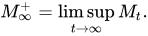
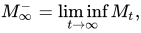
Corollary. (See also Doob's martingale convergence theorems) Let M_t be a continuous martingale, and $M_{\infty }^{-}=\liminf _{t\to \infty }M_{t},$ $M_{\infty }^{+}=\limsup _{t\to \infty }M_{t}.$

Then only the following two cases are possible: $-\infty <M_{\infty }^{-}=M_{\infty }^{+}<+\infty ,$ $-\infty =M_{\infty }^{-}<M_{\infty }^{+}=+\infty ;$ other cases (such as ${\textstyle M_{\infty }^{-}=M_{\infty }^{+}=+\infty ,$ ${\textstyle M_{\infty }^{-}<M_{\infty }^{+}<+\infty$ etc.) are of probability 0.

Especially, a nonnegative continuous martingale has a finite limit (as t → ∞) almost surely.

All stated (in this subsection) for martingales holds also for local martingales.

Change of measure

A wide class of continuous semimartingales (especially, of diffusion processes) is related to the Wiener process via a combination of time change and change of measure.

Using this fact, the qualitative properties stated above for the Wiener process can be generalized to a wide class of continuous semimartingales.

Complex-valued Wiener process

The complex-valued Wiener process may be defined as a complex-valued random process of the form ${\textstyle Z_{t}=X_{t}+iY_{t}$ where ${\textstyle X_{t}$ and ${\textstyle Y_{t}$ are independent Wiener processes (real-valued). In other words, it is the 2-dimensional Wiener process, where we identify ${\textstyle \mathbb {R} ^{2}$ with ${\textstyle \mathbb {C}$ .

Self-similarity

Brownian scaling, time reversal, time inversion: the same as in the real-valued case.

Rotation invariance: for every complex number ${\textstyle c$ such that ${\textstyle |c|=1$ the process ${\textstyle c\cdot Z_{t}$ is another complex-valued Wiener process.

Time change

If ${\textstyle f$ is an entire function then the process ${\textstyle f(Z_{t})-f(0)$ is a time-changed complex-valued Wiener process.

Example: ${\textstyle Z_{t}^{2}=\left(X_{t}^{2}-Y_{t}^{2}\right)+2X_{t}Y_{t}i=U_{A(t)}$ where $A(t)=4\int _{0}^{t}|Z_{s}|^{2}\,\mathrm {d} s$ and ${\textstyle U$ is another complex-valued Wiener process.

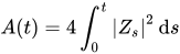
In contrast to the real-valued case, a complex-valued martingale is generally not a time-changed complex-valued Wiener process. For example, the martingale ${\textstyle 2X_{t}+iY_{t}$ is not (here ${\textstyle X_{t}$ and ${\textstyle Y_{t}$ are independent Wiener processes, as before).

Brownian sheet

The Brownian sheet is a multiparamateric generalization. The definition varies from authors, some define the Brownian sheet to have specifically a two-dimensional time parameter ${\textstyle t$ while others define it for general dimensions.

2D Wiener processes with drift (blue) and without drift (red)

08General references

Karatzas, Ioannis; Shreve, Steven E. (1998). Brownian Motion and Stochastic Calculus (2nd ed.). Springer. ISBN 978-0-387-97655-6.
Klenke, Achim (2020). "Brownian Motion". Probability Theory (3rd ed.). Springer. ISBN 978-3-030-56401-8.
Le Gall, Jean-François (2016). Brownian Motion, Martingales, and Stochastic Calculus. Graduate Texts in Mathematics. Vol. 274. Springer. ISBN 978-3-319-31088-6.
Revuz, Daniel; Yor, Marc (2005). Continuous Martingales and Brownian Motion. A Series of Comprehensive Studies in Mathematics. Vol. 293 (3rd ed.). Springer. ISBN 978-3-642-08400-3.

Watch videos about Wiener processExplainers and documentaries on YouTube (opens in a new tab)

Sources and credits

This article is adapted from the Wikipedia article “Wiener process”, written by its contributors and licensed under CC BY-SA 4.0. Fathomly has changed the layout, removed citation markers, navigation and maintenance notices, and adjusted punctuation. This adapted version is shared under the same license. For references, see the original article.

Images, from Wikimedia Commons:

Wiener process with sigma.svg by Unknown author, CC BY-SA 4.0
Wiener process zoom.png by Unknown author, CC BY-SA 3.0
WienerProcess3D.svg by Shiyu Ji, CC BY-SA 4.0
Wiener-process-5traces.svg by Geek3, CC BY-SA 4.0
Wiener process animated.gif by Cyp, CC BY-SA 3.0
BMonSphere.jpg by Thomas Steiner, CC BY-SA 2.5
DriftedWienerProcess1D.svg by Shiyu Ji, CC BY-SA 4.0
ItoWienerProcess2D.svg by Shiyu Ji, CC BY-SA 4.0

Fathomly is not affiliated with or endorsed by the Wikimedia Foundation. Spotted a problem? Tell us.

Wiener process

01Definitions

Canonical definition

Lévy characterization

Gaussian process characterization

Wiener representation

White noise representation

Donsker's theorem: Wiener process as a limit of a random walk

02Properties of a one-dimensional Wiener process

Basic properties

Covariance and correlation

Infinitesimal generator

Running maximum

Arcsine laws

First arcsine law

Second arcsine law

Third arcsine law

Self-similarity

Brownian scaling

Time reversal

Time inversion

Projective invariance

Conformal invariance in two dimensions

Stopping times

Hitting time of level sets

Exit time of intervals

Hitting times of two level sets

A class of Brownian martingales

Properties of sample paths

Qualitative properties

Quantitative properties

Law of the iterated logarithm

Modulus of continuity

Dimension doubling theorem

Local time

Information rate

03d-dimensional Wiener process

Definition

Lévy characterization

Generator representation

04Properties of a d-dimensional Wiener process

Path properties

Infinitesimal generator

Harmonic measure on the sphere

Occupation time formula

Representation of harmonic functions

Stopping times

Moments of exit times

Distribution of exit time from a ball

05Wiener process on Riemannian manifolds

06Infinite dimensional Wiener process

Q-Wiener process

Cylindrical Wiener process

07Related processes

Wiener process with drift

Brownian bridge

Geometric Brownian motion

Ornstein-Uhlenbeck process

Integrated Brownian motion

Process of times to first hitting

Local time

Brownian martingales

Time change

Change of measure

Complex-valued Wiener process

Self-similarity

Time change

Brownian sheet

08General references

Sources and credits

Related topics

Abstract Wiener space

Classical Wiener space

Chernoff's distribution