Encyclopedia

Struve function

Mathematical function

Wikipedia contributorsAdapted for Fathomly · View authors

1 min read
Source updated May 23, 2026

In mathematics, the Struve functions H_α(x), are solutions y(x) of the non-homogeneous Bessel's differential equation:

$x^{2}{\frac {d^{2}y}{dx^{2}}}+x{\frac {dy}{dx}}+\left(x^{2}-\alpha ^{2}\right)y={\frac {4\left({\frac {x}{2}}\right)^{\alpha +1}}{{\sqrt {\pi }}\Gamma \left(\alpha +{\frac {1}{2}}\right)}}$

introduced by Hermann Struve (1882). The complex number α is the order of the Struve function, and is often an integer.

And further defined its second-kind version $\mathbf {K} _{\alpha }(x)$ as $\mathbf {K} _{\alpha }(x)=\mathbf {H} _{\alpha }(x)-Y_{\alpha }(x)$ , where $Y_{\alpha }(x)$ is the Neumann function.

The modified Struve functions L_α(x) are equal to −ie^{−iαπ / 2}H_α(ix) and are solutions y(x) of the non-homogeneous Bessel's differential equation:

$x^{2}{\frac {d^{2}y}{dx^{2}}}+x{\frac {dy}{dx}}-\left(x^{2}+\alpha ^{2}\right)y={\frac {4\left({\frac {x}{2}}\right)^{\alpha +1}}{{\sqrt {\pi }}\Gamma \left(\alpha +{\frac {1}{2}}\right)}}$

And further defined its second-kind version $\mathbf {M} _{\alpha }(x)$ as $\mathbf {M} _{\alpha }(x)=\mathbf {L} _{\alpha }(x)-I_{\alpha }(x)$ , where $I_{\alpha }(x)$ is the modified Bessel function of the first kind.

01Definitions

Since this is a non-homogeneous equation, solutions can be constructed from a single particular solution by adding the solutions of the homogeneous problem. In this case, the homogeneous solutions are the Bessel functions, and the particular solution may be chosen as the corresponding Struve function.

Power series expansion

Struve functions, denoted as H_α(z) have the power series form

$\mathbf {H} _{\alpha }(z)=\sum _{m=0}^{\infty }{\frac {(-1)^{m}}{\Gamma \left(m+{\frac {3}{2}}\right)\Gamma \left(m+\alpha +{\frac {3}{2}}\right)}}\left({\frac {z}{2}}\right)^{2m+\alpha +1},$

where Γ(z) is the gamma function.

The modified Struve functions, denoted L_α(z), have the following power series form

$\mathbf {L} _{\alpha }(z)=\sum _{m=0}^{\infty }{\frac {1}{\Gamma \left(m+{\frac {3}{2}}\right)\Gamma \left(m+\alpha +{\frac {3}{2}}\right)}}\left({\frac {z}{2}}\right)^{2m+\alpha +1}.$

Integral form

Another definition of the Struve function, for values of α satisfying Re(α) > − ⁠1/2⁠, is possible expressing in term of the Poisson's integral representation:

$\mathbf {H} _{\alpha }(x)={\frac {2\left({\frac {x}{2}}\right)^{\alpha }}{{\sqrt {\pi }}\Gamma \left(\alpha +{\frac {1}{2}}\right)}}\int _{0}^{1}(1-t^{2})^{\alpha -{\frac {1}{2}}}\sin xt~dt={\frac {2\left({\frac {x}{2}}\right)^{\alpha }}{{\sqrt {\pi }}\Gamma \left(\alpha +{\frac {1}{2}}\right)}}\int _{0}^{\frac {\pi }{2}}\sin(x\cos \tau )\sin ^{2\alpha }\tau ~d\tau ={\frac {2\left({\frac {x}{2}}\right)^{\alpha }}{{\sqrt {\pi }}\Gamma \left(\alpha +{\frac {1}{2}}\right)}}\int _{0}^{\frac {\pi }{2}}\sin(x\sin \tau )\cos ^{2\alpha }\tau ~d\tau$

$\mathbf {K} _{\alpha }(x)={\frac {2\left({\frac {x}{2}}\right)^{\alpha }}{{\sqrt {\pi }}\Gamma \left(\alpha +{\frac {1}{2}}\right)}}\int _{0}^{\infty }(1+t^{2})^{\alpha -{\frac {1}{2}}}e^{-xt}~dt={\frac {2\left({\frac {x}{2}}\right)^{\alpha }}{{\sqrt {\pi }}\Gamma \left(\alpha +{\frac {1}{2}}\right)}}\int _{0}^{\infty }e^{-x\sinh \tau }\cosh ^{2\alpha }\tau ~d\tau$

$\mathbf {L} _{\alpha }(x)={\frac {2\left({\frac {x}{2}}\right)^{\alpha }}{{\sqrt {\pi }}\Gamma \left(\alpha +{\frac {1}{2}}\right)}}\int _{0}^{1}(1-t^{2})^{\alpha -{\frac {1}{2}}}\sinh xt~dt={\frac {2\left({\frac {x}{2}}\right)^{\alpha }}{{\sqrt {\pi }}\Gamma \left(\alpha +{\frac {1}{2}}\right)}}\int _{0}^{\frac {\pi }{2}}\sinh(x\cos \tau )\sin ^{2\alpha }\tau ~d\tau ={\frac {2\left({\frac {x}{2}}\right)^{\alpha }}{{\sqrt {\pi }}\Gamma \left(\alpha +{\frac {1}{2}}\right)}}\int _{0}^{\frac {\pi }{2}}\sinh(x\sin \tau )\cos ^{2\alpha }\tau ~d\tau$

$\mathbf {M} _{\alpha }(x)=-{\frac {2\left({\frac {x}{2}}\right)^{\alpha }}{{\sqrt {\pi }}\Gamma \left(\alpha +{\frac {1}{2}}\right)}}\int _{0}^{1}(1-t^{2})^{\alpha -{\frac {1}{2}}}e^{-xt}~dt=-{\frac {2\left({\frac {x}{2}}\right)^{\alpha }}{{\sqrt {\pi }}\Gamma \left(\alpha +{\frac {1}{2}}\right)}}\int _{0}^{\frac {\pi }{2}}e^{-x\cos \tau }\sin ^{2\alpha }\tau ~d\tau =-{\frac {2\left({\frac {x}{2}}\right)^{\alpha }}{{\sqrt {\pi }}\Gamma \left(\alpha +{\frac {1}{2}}\right)}}\int _{0}^{\frac {\pi }{2}}e^{-x\sin \tau }\cos ^{2\alpha }\tau ~d\tau$

02Asymptotic forms

For small x, the power series expansion is given above.

For large x, one obtains:

$\mathbf {H} _{\alpha }(x)-Y_{\alpha }(x)={\frac {\left({\frac {x}{2}}\right)^{\alpha -1}}{{\sqrt {\pi }}\Gamma \left(\alpha +{\frac {1}{2}}\right)}}+O\left(\left({\tfrac {x}{2}}\right)^{\alpha -3}\right),$

where Y_α(x) is the Neumann function.

03Properties

The Struve functions satisfy the following recurrence relations:

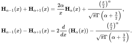
${\begin{aligned}\mathbf {H} _{\alpha -1}(x)+\mathbf {H} _{\alpha +1}(x)&={\frac {2\alpha }{x}}\mathbf {H} _{\alpha }(x)+{\frac {\left({\frac {x}{2}}\right)^{\alpha }}{{\sqrt {\pi }}\Gamma \left(\alpha +{\frac {3}{2}}\right)}},\\\mathbf {H} _{\alpha -1}(x)-\mathbf {H} _{\alpha +1}(x)&=2{\frac {d}{dx}}\left(\mathbf {H} _{\alpha }(x)\right)-{\frac {\left({\frac {x}{2}}\right)^{\alpha }}{{\sqrt {\pi }}\Gamma \left(\alpha +{\frac {3}{2}}\right)}}.\end{aligned}}$

04Relation to other functions

Struve functions of integer order can be expressed in terms of Weber functions E_n and vice versa: if n is a non-negative integer then

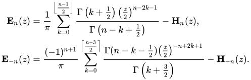
${\begin{aligned}\mathbf {E} _{n}(z)&={\frac {1}{\pi }}\sum _{k=0}^{\left\lfloor {\frac {n-1}{2}}\right\rfloor }{\frac {\Gamma \left(k+{\frac {1}{2}}\right)\left({\frac {z}{2}}\right)^{n-2k-1}}{\Gamma \left(n-k+{\frac {1}{2}}\right)}}-\mathbf {H} _{n}(z),\\\mathbf {E} _{-n}(z)&={\frac {(-1)^{n+1}}{\pi }}\sum _{k=0}^{\left\lceil {\frac {n-3}{2}}\right\rceil }{\frac {\Gamma (n-k-{\frac {1}{2}})\left({\frac {z}{2}}\right)^{-n+2k+1}}{\Gamma \left(k+{\frac {3}{2}}\right)}}-\mathbf {H} _{-n}(z).\end{aligned}}$

Struve functions of order n + ⁠1/2⁠ where n is an integer can be expressed in terms of elementary functions. In particular if n is a non-negative integer then

$\mathbf {H} _{-n-{\frac {1}{2}}}(z)=(-1)^{n}J_{n+{\frac {1}{2}}}(z),$

where the right hand side is a spherical Bessel function.

Struve functions (of any order) can be expressed in terms of the generalized hypergeometric function ₁F₂:

$\mathbf {H} _{\alpha }(z)={\frac {z^{\alpha +1}}{2^{\alpha }{\sqrt {\pi }}\Gamma \left(\alpha +{\tfrac {3}{2}}\right)}}{}_{1}F_{2}\left(1;{\tfrac {3}{2}},\alpha +{\tfrac {3}{2}};-{\tfrac {z^{2}}{4}}\right).$

05Applications

The Struve and Weber functions were shown to have an application to beamforming in., and in describing the effect of confining interface on Brownian motion of colloidal particles at low Reynolds numbers.

Watch videos about Struve functionExplainers and documentaries on YouTube (opens in a new tab)

Sources and credits

This article is adapted from the Wikipedia article “Struve function”, written by its contributors and licensed under CC BY-SA 4.0. Fathomly has changed the layout, removed citation markers, navigation and maintenance notices, and adjusted punctuation. This adapted version is shared under the same license. For references, see the original article.

Images, from Wikimedia Commons:

Fathomly is not affiliated with or endorsed by the Wikimedia Foundation. Spotted a problem? Tell us.