Reference articles on history, science, culture and more
Encyclopedia

Stochastic dynamic programming

1957 technique for modelling problems of decision making under uncertainty

Originally introduced by Richard E. Bellman in (Bellman 1957), stochastic dynamic programming (SDP) is a technique for modelling and solving problems of decision making under uncertainty. Closely related to stochastic programming and dynamic programming, stochastic dynamic programming represents the problem under scrutiny in the form of a Bellman equation. The aim is to compute a policy prescribing how to act optimally in the face of uncertainty.

01A motivating example: Gambling game

A gambler has $2, she is allowed to play a game of chance 4 times and her goal is to maximize her probability of ending up with a least $6. If the gambler bets $b on a play of the game, then with probability 0.4 she wins the game, recoups the initial bet, and she increases her capital position by $b; with probability 0.6, she loses the bet amount $b; all plays are pairwise independent. On any play of the game, the gambler may not bet more money than she has available at the beginning of that play.

Stochastic dynamic programming can be employed to model this problem and determine a betting strategy that, for instance, maximizes the gambler's probability of attaining a wealth of at least $6 by the end of the betting horizon.

Note that if there is no limit to the number of games that can be played, the problem becomes a variant of the well known St. Petersburg paradox.

An optimal betting strategy that maximizes the gambler's probability of attaining a wealth of at least $6 by the end of the betting horizon; represents the bet amount for game when the gambler has $ at the beginning of that play. If the decision maker follows this policy, with probability 0.1984 she will attain a wealth of at least $6.

02Formal background

Consider a discrete system defined on n stages in which each stage t=1,\ldots ,n is characterized by

  • an initial state s_{t}\in S_{t}, where S_{t} is the set of feasible states at the beginning of stage t;
  • a decision variable x_{t}\in X_{t}, where X_{t} is the set of feasible actions at stage t, note that X_{t} may be a function of the initial state s_{t};
  • an immediate cost/reward function p_{t}(s_{t},x_{t}), representing the cost/reward at stage t if s_{t} is the initial state and x_{t} the action selected;
  • a state transition function g_{t}(s_{t},x_{t}) that leads the system towards state s_{t+1}=g_{t}(s_{t},x_{t}).

Let f_{t}(s_{t}) represent the optimal cost/reward obtained by following an optimal policy over stages t,t+1,\ldots ,n. Without loss of generality in what follow we will consider a reward maximisation setting. In deterministic dynamic programming one usually deals with functional equations taking the following structure

f_{t}(s_{t})=\max _{x_{t}\in X_{t}}\{p_{t}(s_{t},x_{t})+f_{t+1}(s_{t+1})\}

where s_{t+1}=g_{t}(s_{t},x_{t}) and the boundary condition of the system is

f_{n}(s_{n})=\max _{x_{n}\in X_{n}}\{p_{n}(s_{n},x_{n})\}.

The aim is to determine the set of optimal actions that maximise f_{1}(s_{1}). Given the current state s_{t} and the current action x_{t}, we know with certainty the reward secured during the current stage and, thanks to the state transition function g_{t}, the future state towards which the system transitions.

In practice, however, even if we know the state of the system at the beginning of the current stage as well as the decision taken, the state of the system at the beginning of the next stage and the current period reward are often random variables that can be observed only at the end of the current stage.

Stochastic dynamic programming deals with problems in which the current period reward and/or the next period state are random, i.e. with multi-stage stochastic systems. The decision maker's goal is to maximise expected (discounted) reward over a given planning horizon.

In their most general form, stochastic dynamic programs deal with functional equations taking the following structure

f_{t}(s_{t})=\max _{x_{t}\in X_{t}(s_{t})}\left\{({\text{expected reward during stage }}t\mid s_{t},x_{t})+\alpha \sum _{s_{t+1}}\Pr(s_{t+1}\mid s_{t},x_{t})f_{t+1}(s_{t+1})\right\}

where

  • f_{t}(s_{t}) is the maximum expected reward that can be attained during stages t,t+1,\ldots ,n, given state s_{t} at the beginning of stage t;
  • x_{t} belongs to the set X_{t}(s_{t}) of feasible actions at stage t given initial state s_{t};
  • \alpha is the discount factor;
  • \Pr(s_{t+1}\mid s_{t},x_{t}) is the conditional probability that the state at the end of stage t is s_{t+1} given current state s_{t} and selected action x_{t}.

Markov decision processes represent a special class of stochastic dynamic programs in which the underlying stochastic process has state transitions satisfying the Markov property.

Gambling game as a stochastic dynamic program

Gambling game can be formulated as a Stochastic Dynamic Program as follows: there are n=4 games (i.e. stages) in the planning horizon

  • the state s in period t represents the initial wealth at the beginning of period t;
  • the action given state s in period t is the bet amount b;
  • the transition probability p_{i,j}^{a} from state i to state j when action a is taken in state i is easily derived from the probability of winning (0.4) or losing (0.6) a game.

Let f_{t}(s) be the probability that, by the end of game 4, the gambler has at least $6, given that she has $s at the beginning of game t.

  • the immediate profit incurred if action b is taken in state s is given by the expected value p_{t}(s,b)=0.4f_{t+1}(s+b)+0.6f_{t+1}(s-b).

To derive the functional equation, define b_{t}(s) as a bet that attains f_{t}(s), then at the beginning of game t=4

  • if s<3 it is impossible to attain the goal, i.e. f_{4}(s)=0 for s<3;
  • if s\geq 6 the goal is attained, i.e. f_{4}(s)=1 for s\geq 6;
  • if 3\leq s\leq 5 the gambler should bet enough to attain the goal, i.e. f_{4}(s)=0.4 for 3\leq s\leq 5.

For t<4 the functional equation is f_{t}(s)=\max _{b_{t}(s)}\{0.4f_{t+1}(s+b)+0.6f_{t+1}(s-b)\}, where b_{t}(s) ranges in 0,...,s; the aim is to find f_{1}(2).

Given the functional equation, an optimal betting policy can be obtained via forward recursion or backward recursion algorithms, as outlined below.

03Solution methods

Stochastic dynamic programs can be solved to optimality by using backward recursion or forward recursion algorithms. Memoization is typically employed to enhance performance. However, like deterministic dynamic programming also its stochastic variant suffers from the curse of dimensionality. For this reason approximate solution methods are typically employed in practical applications.

Backward recursion

Given a bounded state space, backward recursion (Bertsekas 2000) begins by tabulating f_{n}(k) for every possible state k belonging to the final stage n. Once these values are tabulated, together with the associated optimal state-dependent actions x_{n}(k), it is possible to move to stage n-1 and tabulate f_{n-1}(k) for all possible states belonging to the stage n-1. The process continues by considering in a backward fashion all remaining stages up to the first one. Once this tabulation process is complete, f_{1}(s), the value of an optimal policy given initial state s, as well as the associated optimal action x_{1}(s) can be easily retrieved from the table. Since the computation proceeds in a backward fashion, it is clear that backward recursion may lead to computation of a large number of states that are not necessary for the computation of f_{1}(s).

Example: Gambling game

Forward recursion

Given the initial state s of the system at the beginning of period 1, forward recursion (Bertsekas 2000) computes f_{1}(s) by progressively expanding the functional equation (forward pass). This involves recursive calls for all f_{t+1}(\cdot ),f_{t+2}(\cdot ),\ldots that are necessary for computing a given f_{t}(\cdot ). The value of an optimal policy and its structure are then retrieved via a (backward pass) in which these suspended recursive calls are resolved. A key difference from backward recursion is the fact that f_{t} is computed only for states that are relevant for the computation of f_{1}(s). Memoization is employed to avoid recomputation of states that have been already considered.

Example: Gambling game

We shall illustrate forward recursion in the context of the Gambling game instance previously discussed. We begin the forward pass by considering f_{1}(2)=\min \left\{{\begin{array}{rr}b&{\text{success probability in periods 1,2,3,4}}\\\hline 0&0.4f_{2}(2+0)+0.6f_{2}(2-0)\\1&0.4f_{2}(2+1)+0.6f_{2}(2-1)\\2&0.4f_{2}(2+2)+0.6f_{2}(2-2)\\\end{array}}\right.
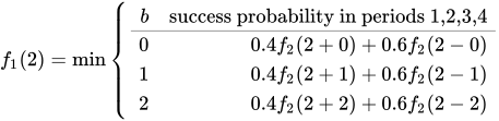
At this point we have not computed yet f_{2}(4),f_{2}(3),f_{2}(2),f_{2}(1),f_{2}(0), which are needed to compute f_{1}(2); we proceed and compute these items. Note that f_{2}(2+0)=f_{2}(2-0)=f_{2}(2), therefore one can leverage memoization and perform the necessary computations only once.

Computation of f_{2}(4),f_{2}(3),f_{2}(2),f_{2}(1),f_{2}(0)

f_{2}(0)=\min \left\{{\begin{array}{rr}b&{\text{success probability in periods 2,3,4}}\\\hline 0&0.4f_{3}(0+0)+0.6f_{3}(0-0)\\\end{array}}\right.

f_{2}(1)=\min \left\{{\begin{array}{rr}b&{\text{success probability in periods 2,3,4}}\\\hline 0&0.4f_{3}(1+0)+0.6f_{3}(1-0)\\1&0.4f_{3}(1+1)+0.6f_{3}(1-1)\\\end{array}}\right.

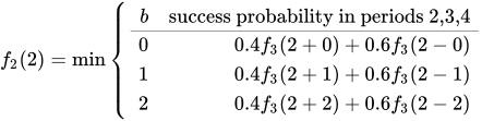
f_{2}(2)=\min \left\{{\begin{array}{rr}b&{\text{success probability in periods 2,3,4}}\\\hline 0&0.4f_{3}(2+0)+0.6f_{3}(2-0)\\1&0.4f_{3}(2+1)+0.6f_{3}(2-1)\\2&0.4f_{3}(2+2)+0.6f_{3}(2-2)\\\end{array}}\right.

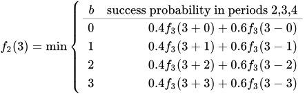
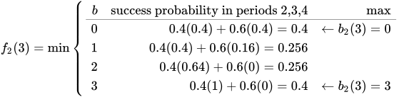
f_{2}(3)=\min \left\{{\begin{array}{rr}b&{\text{success probability in periods 2,3,4}}\\\hline 0&0.4f_{3}(3+0)+0.6f_{3}(3-0)\\1&0.4f_{3}(3+1)+0.6f_{3}(3-1)\\2&0.4f_{3}(3+2)+0.6f_{3}(3-2)\\3&0.4f_{3}(3+3)+0.6f_{3}(3-3)\\\end{array}}\right.

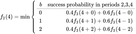
f_{2}(4)=\min \left\{{\begin{array}{rr}b&{\text{success probability in periods 2,3,4}}\\\hline 0&0.4f_{3}(4+0)+0.6f_{3}(4-0)\\1&0.4f_{3}(4+1)+0.6f_{3}(4-1)\\2&0.4f_{3}(4+2)+0.6f_{3}(4-2)\end{array}}\right.

We have now computed f_{2}(k) for all k that are needed to compute f_{1}(2). However, this has led to additional suspended recursions involving f_{3}(4),f_{3}(3),f_{3}(2),f_{3}(1),f_{3}(0). We proceed and compute these values.

Computation of f_{3}(4),f_{3}(3),f_{3}(2),f_{3}(1),f_{3}(0)

f_{3}(0)=\min \left\{{\begin{array}{rr}b&{\text{success probability in periods 3,4}}\\\hline 0&0.4f_{4}(0+0)+0.6f_{4}(0-0)\\\end{array}}\right.

f_{3}(1)=\min \left\{{\begin{array}{rr}b&{\text{success probability in periods 3,4}}\\\hline 0&0.4f_{4}(1+0)+0.6f_{4}(1-0)\\1&0.4f_{4}(1+1)+0.6f_{4}(1-1)\\\end{array}}\right.

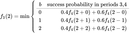
f_{3}(2)=\min \left\{{\begin{array}{rr}b&{\text{success probability in periods 3,4}}\\\hline 0&0.4f_{4}(2+0)+0.6f_{4}(2-0)\\1&0.4f_{4}(2+1)+0.6f_{4}(2-1)\\2&0.4f_{4}(2+2)+0.6f_{4}(2-2)\\\end{array}}\right.

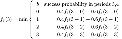
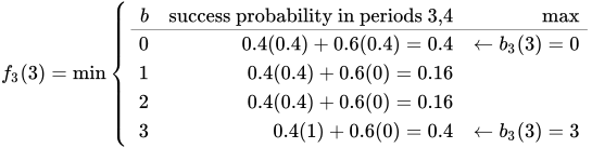
f_{3}(3)=\min \left\{{\begin{array}{rr}b&{\text{success probability in periods 3,4}}\\\hline 0&0.4f_{4}(3+0)+0.6f_{4}(3-0)\\1&0.4f_{4}(3+1)+0.6f_{4}(3-1)\\2&0.4f_{4}(3+2)+0.6f_{4}(3-2)\\3&0.4f_{4}(3+3)+0.6f_{4}(3-3)\\\end{array}}\right.

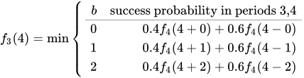
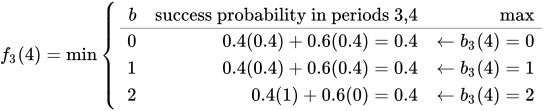
f_{3}(4)=\min \left\{{\begin{array}{rr}b&{\text{success probability in periods 3,4}}\\\hline 0&0.4f_{4}(4+0)+0.6f_{4}(4-0)\\1&0.4f_{4}(4+1)+0.6f_{4}(4-1)\\2&0.4f_{4}(4+2)+0.6f_{4}(4-2)\end{array}}\right.

f_{3}(5)=\min \left\{{\begin{array}{rr}b&{\text{success probability in periods 3,4}}\\\hline 0&0.4f_{4}(5+0)+0.6f_{4}(5-0)\\1&0.4f_{4}(5+1)+0.6f_{4}(5-1)\end{array}}\right.

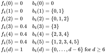
Since stage 4 is the last stage in our system, f_{4}(\cdot ) represent boundary conditions that are easily computed as follows.

Boundary conditions

{\begin{array}{ll}f_{4}(0)=0&b_{4}(0)=0\\f_{4}(1)=0&b_{4}(1)=\{0,1\}\\f_{4}(2)=0&b_{4}(2)=\{0,1,2\}\\f_{4}(3)=0.4&b_{4}(3)=\{3\}\\f_{4}(4)=0.4&b_{4}(4)=\{2,3,4\}\\f_{4}(5)=0.4&b_{4}(5)=\{1,2,3,4,5\}\\f_{4}(d)=1&b_{4}(d)=\{0,\ldots ,d-6\}{\text{ for }}d\geq 6\end{array}}

At this point it is possible to proceed and recover the optimal policy and its value via a backward pass involving, at first, stage 3

Backward pass involving f_{3}(\cdot )

f_{3}(0)=\min \left\{{\begin{array}{rr}b&{\text{success probability in periods 3,4}}\\\hline 0&0.4(0)+0.6(0)=0\\\end{array}}\right.

f_{3}(1)=\min \left\{{\begin{array}{rrr}b&{\text{success probability in periods 3,4}}&{\mbox{max}}\\\hline 0&0.4(0)+0.6(0)=0&\leftarrow b_{3}(1)=0\\1&0.4(0)+0.6(0)=0&\leftarrow b_{3}(1)=1\\\end{array}}\right.

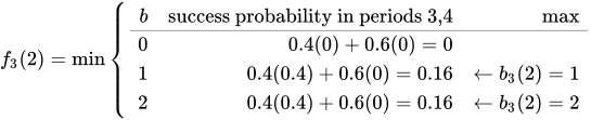
f_{3}(2)=\min \left\{{\begin{array}{rrr}b&{\text{success probability in periods 3,4}}&{\mbox{max}}\\\hline 0&0.4(0)+0.6(0)=0\\1&0.4(0.4)+0.6(0)=0.16&\leftarrow b_{3}(2)=1\\2&0.4(0.4)+0.6(0)=0.16&\leftarrow b_{3}(2)=2\\\end{array}}\right.

f_{3}(3)=\min \left\{{\begin{array}{rrr}b&{\text{success probability in periods 3,4}}&{\mbox{max}}\\\hline 0&0.4(0.4)+0.6(0.4)=0.4&\leftarrow b_{3}(3)=0\\1&0.4(0.4)+0.6(0)=0.16\\2&0.4(0.4)+0.6(0)=0.16\\3&0.4(1)+0.6(0)=0.4&\leftarrow b_{3}(3)=3\\\end{array}}\right.

f_{3}(4)=\min \left\{{\begin{array}{rrr}b&{\text{success probability in periods 3,4}}&{\mbox{max}}\\\hline 0&0.4(0.4)+0.6(0.4)=0.4&\leftarrow b_{3}(4)=0\\1&0.4(0.4)+0.6(0.4)=0.4&\leftarrow b_{3}(4)=1\\2&0.4(1)+0.6(0)=0.4&\leftarrow b_{3}(4)=2\\\end{array}}\right.

f_{3}(5)=\min \left\{{\begin{array}{rrr}b&{\text{success probability in periods 3,4}}&{\mbox{max}}\\\hline 0&0.4(0.4)+0.6(0.4)=0.4\\1&0.4(1)+0.6(0.4)=0.64&\leftarrow b_{3}(5)=1\\\end{array}}\right.

and, then, stage 2.

Backward pass involving f_{2}(\cdot )

f_{2}(0)=\min \left\{{\begin{array}{rrr}b&{\text{success probability in periods 2,3,4}}&{\mbox{max}}\\\hline 0&0.4(0)+0.6(0)=0&\leftarrow b_{2}(0)=0\\\end{array}}\right.

f_{2}(1)=\min \left\{{\begin{array}{rrr}b&{\text{success probability in periods 2,3,4}}&{\mbox{max}}\\\hline 0&0.4(0)+0.6(0)=0\\1&0.4(0.16)+0.6(0)=0.064&\leftarrow b_{2}(1)=1\\\end{array}}\right.

f_{2}(2)=\min \left\{{\begin{array}{rrr}b&{\text{success probability in periods 2,3,4}}&{\mbox{max}}\\\hline 0&0.4(0.16)+0.6(0.16)=0.16&\leftarrow b_{2}(2)=0\\1&0.4(0.4)+0.6(0)=0.16&\leftarrow b_{2}(2)=1\\2&0.4(0.4)+0.6(0)=0.16&\leftarrow b_{2}(2)=2\\\end{array}}\right.

f_{2}(3)=\min \left\{{\begin{array}{rrr}b&{\text{success probability in periods 2,3,4}}&{\mbox{max}}\\\hline 0&0.4(0.4)+0.6(0.4)=0.4&\leftarrow b_{2}(3)=0\\1&0.4(0.4)+0.6(0.16)=0.256\\2&0.4(0.64)+0.6(0)=0.256\\3&0.4(1)+0.6(0)=0.4&\leftarrow b_{2}(3)=3\\\end{array}}\right.

f_{2}(4)=\min \left\{{\begin{array}{rrr}b&{\text{success probability in periods 2,3,4}}&{\mbox{max}}\\\hline 0&0.4(0.4)+0.6(0.4)=0.4\\1&0.4(0.64)+0.6(0.4)=0.496&\leftarrow b_{2}(4)=1\\2&0.4(1)+0.6(0.16)=0.496&\leftarrow b_{2}(4)=2\\\end{array}}\right.

We finally recover the value f_{1}(2) of an optimal policy

f_{1}(2)=\min \left\{{\begin{array}{rrr}b&{\text{success probability in periods 1,2,3,4}}&{\mbox{max}}\\\hline 0&0.4(0.16)+0.6(0.16)=0.16\\1&0.4(0.4)+0.6(0.064)=0.1984&\leftarrow b_{1}(2)=1\\2&0.4(0.496)+0.6(0)=0.1984&\leftarrow b_{1}(2)=2\\\end{array}}\right.

This is the optimal policy that has been previously illustrated. Note that there are multiple optimal policies leading to the same optimal value f_{1}(2)=0.1984; for instance, in the first game one may either bet $1 or $2.

Python implementation. The one that follows is a complete Python implementation of this example.

import functools class memoize: def __init__(self, func): self.func = func self.memoized = {} self.method_cache = {} def __call__(self, *args): return self.cache_get(self.memoized, args, lambda: self.func(*args)) def __get__(self, obj, objtype): return self.cache_get( self.method_cache, obj, lambda: self.__class__(functools.partial(self.func, obj)), ) def cache_get(self, cache, key, func): try: return cache[key] except KeyError: cache[key] = func() return cache[key] def reset(self): self.memoized = {} self.method_cache = {} class State: """The state of the gambler's ruin problem""" def __init__(self, t: int, wealth: float): """state constructor Arguments: t {int} -- time period wealth {float} -- initial wealth """ self.t, self.wealth = t, wealth def __eq__(self, other): return self.__dict__ == other.__dict__ def __str__(self): return str(self.t) + " " + str(self.wealth) def __hash__(self): return hash(str(self)) class GamblersRuin: def __init__( self, bettingHorizon: int, targetWealth: float, pmf: list[list[tuple[int, float]]], ): """The gambler's ruin problem. Arguments: bettingHorizon {int} -- betting horizon targetWealth {float} -- target wealth pmf {list[list[tuple[int, float]]]} -- probability mass function """ # initialize instance variables self.bettingHorizon, self.targetWealth, self.pmf = ( bettingHorizon, targetWealth, pmf, ) # lambdas self.ag = lambda s: [ i for i in range(0, min(self.targetWealth // 2, s.wealth) + 1) ] # action generator self.st = lambda s, a, r: State( s.t + 1, s.wealth - a + a * r ) # state transition self.iv = ( lambda s, a, r: 1 if s.wealth - a + a * r >= self.targetWealth else 0 ) # immediate value function self.cache_actions = {} # cache with optimal state/action pairs def f(self, wealth: float) -> float: s = State(0, wealth) return self._f(s) def q(self, t: int, wealth: float) -> float: s = State(t, wealth) return self.cache_actions[str(s)] @memoize def _f(self, s: State) -> float: # Forward recursion values = [sum([p[1]*(self._f(self.st(s, a, p[0])) if s.t < self.bettingHorizon - 1 else self.iv(s, a, p[0])) # value function for p in self.pmf[s.t]]) # bet realisations for a in self.ag(s)] # actions v = max(values) try: self.cache_actions[str(s)] = self.ag(s)[values.index(v)] # store best action except ValueError: self.cache_actions[str(s)] = None print("Error in retrieving best action") return v # return expected total cost instance = { "bettingHorizon": 4, "targetWealth": 6, "pmf": [[(0, 0.6), (2, 0.4)] for i in range(0, 4)], } gr, initial_wealth = GamblersRuin(**instance), 2 # f_1(x) is gambler's probability of attaining $targetWealth at the end of bettingHorizon print("f_1(" + str(initial_wealth) + "): " + str(gr.f(initial_wealth))) # Recover optimal action for period 2 when initial wealth at the beginning of period 2 is $1. t, initial_wealth = 1, 1 print( "b_" + str(t + 1) + "(" + str(initial_wealth) + "): " + str(gr.q(t, initial_wealth)) )

Java implementation. GamblersRuin.java is a standalone Java 8 implementation of the above example.

Approximate dynamic programming

Approximate dynamic programming (ADP) (also known as neuro-dynamic programming or reinforcement learning) is a general approach to modeling and algorithmic strategy, mostly for stochastic problems and sometimes for large and complex problems. ADP, like SDP, was created by Richard Bellman, and later developed (at first independently) by the operations research, computer science, and engineering controls communities. Warren B. Powell wrote in an article in Annals of Operations Research how:

More so than other communities, operations research continued to develop the theory behind the basic model introduced by Bellman with discrete states and actions, even while authors as early as Bellman himself recognized its limits due to the “curse of dimensionality” inherent in discrete state spaces.

The curse of dimensionality (the difficulty in analyzing data with multiple aspect (dimensions)) is a well established issue with the use of Bellman's equation, and ADP is often presented as a method for overcoming this issue. However, the main idea of ADP is "learning what to learn, and how to learn it, to make better decisions over time".

Stochastic dual dynamic programming (SDDP)

One method that can be regarded as an approximate dynamic programming method is stochastic dual dynamic programming (SDDP). M. V. F. Periera and L. V. M. G. Pinto had proposed the idea in 1991 with "a methodology for the solution of multistage stochastic optimization problems, based on the approximation of the expected-cost-to-go functions of stochastic dynamic programming by piecewise linear functions." Their motivation was largely for a more efficient optimization method than stochastic dynamic programming (SDP) for operating Brazilian power plants. Developing in part from stochastic dynamic programming (SDP), SDDP is an algorithm that addresses multistage stochastic problems by means of finding an optimal policy by means of computation or by means of an approximate solution. Along with SDP serving as a foundation to SDDP, stochastic programming also was part of the history of the development of SDDP.

Watch videos about Stochastic dynamic programmingExplainers and documentaries on YouTube (opens in a new tab)

Sources and credits

This article is adapted from the Wikipedia article Stochastic dynamic programming, written by its contributors and licensed under CC BY-SA 4.0. Fathomly has changed the layout, removed citation markers, navigation and maintenance notices, and adjusted punctuation. This adapted version is shared under the same license. For references, see the original article.

Images, from Wikimedia Commons:

Fathomly is not affiliated with or endorsed by the Wikimedia Foundation. Spotted a problem? Tell us.