Encyclopedia

Spectral sequence

Tool in homological algebra

Wikipedia contributorsAdapted for Fathomly · View authors

20 min read
Source updated July 23, 2026

In homological algebra and algebraic topology, a spectral sequence is a means of computing homology groups by taking successive approximations. Spectral sequences are a generalization of exact sequences, and since their introduction by Jean Leray (1946a, 1946b), they have become important computational tools, particularly in algebraic topology, algebraic geometry and homological algebra.

01Discovery and motivation

Motivated by problems in algebraic topology, Jean Leray introduced the notion of a sheaf and found himself faced with the problem of computing sheaf cohomology. To compute sheaf cohomology, Leray introduced a computational technique now known as the Leray spectral sequence. This gave a relation between cohomology groups of a sheaf and cohomology groups of the pushforward of the sheaf. The relation involved an infinite process. Leray found that the cohomology groups of the pushforward formed a natural chain complex, so that he could take the cohomology of the cohomology. This was still not the cohomology of the original sheaf, but it was one step closer in a sense. The cohomology of the cohomology again formed a chain complex, and its cohomology formed a chain complex, and so on. The limit of this infinite process was essentially the same as the cohomology groups of the original sheaf.

It was soon realized that Leray's computational technique was an example of a more general phenomenon. Spectral sequences were found in diverse situations, and they gave intricate relationships among homology and cohomology groups coming from geometric situations such as fibrations and from algebraic situations involving derived functors. While their theoretical importance has decreased since the introduction of derived categories, they are still the most effective computational tool available. This is true even when many of the terms of the spectral sequence are incalculable.

Unfortunately, because of the large amount of information carried in spectral sequences, they are difficult to grasp. This information is usually contained in a rank three lattice of abelian groups or modules. The easiest cases to deal with are those in which the spectral sequence eventually collapses, meaning that going out further in the sequence produces no new information. Even when this does not happen, it is often possible to get useful information from a spectral sequence by various tricks.

02Formal definition

Cohomological spectral sequence

Fix an abelian category, such as a category of modules over a ring, and a nonnegative integer $r_{0}$ . A cohomological spectral sequence is a sequence $\{E_{r},d_{r}\}_{r\geq r_{0}}$ of objects $E_{r}$ and endomorphisms $d_{r}:E_{r}\to E_{r}$ , such that for every $r\geq r_{0}$

$d_{r}\circ d_{r}=0$ ,
$E_{r+1}\cong H_{*}(E_{r},d_{r})$ , the homology of $E_{r}$ with respect to $d_{r}$ .

Usually the isomorphisms are suppressed and we write $E_{r+1}=H_{*}(E_{r},d_{r})$ instead. An object $E_{r}$ is called sheet (as in a sheet of paper), or sometimes a page or a term; an endomorphism $d_{r}$ is called boundary map or differential. Sometimes $E_{r+1}$ is called the derived object of $E_{r}$ .

Bigraded spectral sequence

In reality spectral sequences mostly occur in the category of doubly graded modules over a ring R (or doubly graded sheaves of modules over a sheaf of rings), i.e. every sheet is a bigraded R-module ${\textstyle E_{r}=\bigoplus _{p,q\in \mathbb {Z} ^{2}}E_{r}^{p,q}.$ So in this case a cohomological spectral sequence is a sequence $\{E_{r},d_{r}\}_{r\geq r_{0}}$ of bigraded R-modules $\{E_{r}^{p,q}\}_{p,q}$ and for every module the direct sum of endomorphisms $d_{r}=(d_{r}^{p,q}:E_{r}^{p,q}\to E_{r}^{p+r,q-r+1})_{p,q\in \mathbb {Z} ^{2}}$ of bidegree $(r,1-r)$ , such that for every $r\geq r_{0}$ it holds that:

$d_{r}^{p+r,q-r+1}\circ d_{r}^{p,q}=0$ ,
$E_{r+1}\cong H_{*}(E_{r},d_{r})$ .

The notation used here is called complementary degree. Some authors write $E_{r}^{d,q}$ instead, where $d=p+q$ is the total degree. Depending upon the spectral sequence, the boundary map on the first sheet can have a degree which corresponds to r = 0, r = 1, or r = 2. For example, for the spectral sequence of a filtered complex, described below, r₀ = 0, but for the Grothendieck spectral sequence, r₀ = 2. Usually r₀ is zero, one, or two. In the ungraded situation described above, r₀ is irrelevant.

Homological spectral sequence

Mostly the objects we are talking about are chain complexes, that occur with descending (like above) or ascending order. In the latter case, by replacing $E_{r}^{p,q}$ with $E_{p,q}^{r}$ and $d_{r}^{p,q}:E_{r}^{p,q}\to E_{r}^{p+r,q-r+1}$ with $d_{p,q}^{r}:E_{p,q}^{r}\to E_{p-r,q+r-1}^{r}$ (bidegree $(-r,r-1)$ ), one receives the definition of a homological spectral sequence analogously to the cohomological case.

Spectral sequence from a chain complex

The most elementary example in the ungraded situation is a chain complex C_•. An object C_• in an abelian category of chain complexes naturally comes with a differential d. Let r₀ = 0, and let E₀ be C_•. This forces E₁ to be the complex H(C_•): At the i′th location this is the i′th homology group of C_•. The only natural differential on this new complex is the zero map, so we let d₁ = 0. This forces $E_{2}$ to equal $E_{1}$ , and again our only natural differential is the zero map. Putting the zero differential on all the rest of our sheets gives a spectral sequence whose terms are:

E₀ = C_•
E_r = H(C_•) for all r ≥ 1.

The terms of this spectral sequence stabilize at the first sheet because its only nontrivial differential was on the zeroth sheet. Consequently, we can get no more information at later steps. Usually, to get useful information from later sheets, we need extra structure on the $E_{r}$ .

03Visualization

A doubly graded spectral sequence has a tremendous amount of data to keep track of, but there is a common visualization technique which makes the structure of the spectral sequence clearer. We have three indices, r, p, and q. An object $E_{r}$ can be seen as the r^th checkered page of a book. On these sheets, we will take p to be the horizontal direction and q to be the vertical direction. At each lattice point we have the object $E_{r}^{p,q}$ . Now turning to the next page means taking homology, that is the $(r+1)$ ^th page is a subquotient of the r^th page. The total degree n = p + q runs diagonally, northwest to southeast, across each sheet. In the homological case, the differentials have bidegree (−r, r − 1), so they decrease n by one. In the cohomological case, n is increased by one. The differentials change their direction with each turn with respect to r.

The red arrows demonstrate the case of a first quadrant sequence (see example below), where only the objects of the first quadrant are non-zero. While turning pages, either the domain or the codomain of all the differentials become zero.

04Properties

Categorical properties

The set of cohomological spectral sequences form a category: a morphism of spectral sequences $f:E\to E'$ is by definition a collection of maps $f_{r}:E_{r}\to E'_{r}$ which are compatible with the differentials, i.e. $f_{r}\circ d_{r}=d'_{r}\circ f_{r}$ , and with the given isomorphisms between the cohomology of the r^th step and the ⁠ $(r+1)$ ⁠^th sheets of E and E′, respectively: $f_{r+1}(E_{r+1})\,=\,f_{r+1}(H(E_{r}))\,=\,H(f_{r}(E_{r}))$ . In the bigraded case, they should also respect the graduation: $f_{r}(E_{r}^{p,q})\subset {E'_{r}}^{p,q}.$

Multiplicative structure

A cup product gives a ring structure to a cohomology group, turning it into a cohomology ring. Thus, it is natural to consider a spectral sequence with a ring structure as well. Let $E_{r}^{p,q}$ be a spectral sequence of cohomological type. We say it has multiplicative structure if (i) $E_{r}$ are (doubly graded) differential graded algebras and (ii) the multiplication on $E_{r+1}$ is induced by that on $E_{r}$ via passage to cohomology.

A typical example is the cohomological Serre spectral sequence for a fibration $F\to E\to B$ , when the coefficient group is a ring R. It has the multiplicative structure induced by the cup products of fibre and base on the $E_{2}$ -page. However, in general the limiting term $E_{\infty }$ is not isomorphic as a graded algebra to H(E; R). The multiplicative structure can be very useful for calculating differentials on the sequence.

05Constructions of spectral sequences

Spectral sequences can be constructed by various ways. In algebraic topology, an exact couple is perhaps the most common tool for the construction. In algebraic geometry, spectral sequences are usually constructed from filtrations of cochain complexes.

Spectral sequence of an exact couple

Another technique for constructing spectral sequences is William Massey's method of exact couples. Exact couples are particularly common in algebraic topology. Despite this they are unpopular in abstract algebra, where most spectral sequences come from filtered complexes.

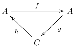
To define exact couples, we begin again with an abelian category. As before, in practice this is usually the category of doubly graded modules over a ring. An exact couple is a pair of objects (A, C), together with three homomorphisms between these objects: f : A → A, g : A → C and h : C → A subject to certain exactness conditions:

Image f = Kernel g
Image g = Kernel h
Image h = Kernel f

We will abbreviate this data by (A, C, f, g, h). Exact couples are usually depicted as triangles. We will see that C corresponds to the E₀ term of the spectral sequence and that A is some auxiliary data.

To pass to the next sheet of the spectral sequence, we will form the derived couple. We set:

d = g o h
A' = f(A)
C' = Ker d / Im d
f ' = f|_A', the restriction of f to A'
h' : C' → A' is induced by h. It is straightforward to see that h induces such a map.
g' : A' → C' is defined on elements as follows: For each a in A', write a as f(b) for some b in A. g'(a) is defined to be the image of g(b) in C'. In general, g' can be constructed using one of the embedding theorems for abelian categories.

From here it is straightforward to check that (A', C', f ', g', h') is an exact couple. C' corresponds to the E₁ term of the spectral sequence. We can iterate this procedure to get exact couples (A⁽ⁿ⁾, C⁽ⁿ⁾, f⁽ⁿ⁾, g⁽ⁿ⁾, h⁽ⁿ⁾).

In order to construct a spectral sequence, let E_n be C⁽ⁿ⁾ and d_n be g⁽ⁿ⁾ o h⁽ⁿ⁾.

Spectral sequences constructed with this method

Serre spectral sequence - used to compute (co)homology of a fibration
Atiyah-Hirzebruch spectral sequence - used to compute (co)homology of extraordinary cohomology theories, such as K-theory
Bockstein spectral sequence.
Spectral sequences of filtered complexes

The spectral sequence of a filtered complex

A very common type of spectral sequence comes from a filtered cochain complex, as it naturally induces a bigraded object. Consider a cochain complex $(C^{\bullet },d)$ together with a descending filtration, ${\textstyle ...\supset \,F^{-2}C^{\bullet }\,\supset \,F^{-1}C^{\bullet }\supset F^{0}C^{\bullet }\,\supset \,F^{1}C^{\bullet }\,\supset \,F^{2}C^{\bullet }\,\supset \,F^{3}C^{\bullet }\,\supset ...\,$ . We require that the boundary map is compatible with the filtration, i.e. ${\textstyle d(F^{p}C^{n})\subset F^{p}C^{n+1}$ , and that the filtration is exhaustive, that is, the union of the set of all ${\textstyle F^{p}C^{\bullet }$ is the entire chain complex ${\textstyle C^{\bullet }$ . Then there exists a spectral sequence with ${\textstyle E_{0}^{p,q}=F^{p}C^{p+q}/F^{p+1}C^{p+q}$ and ${\textstyle E_{1}^{p,q}=H^{p+q}(F^{p}C^{\bullet }/F^{p+1}C^{\bullet })$ . Later, we will also assume that the filtration is Hausdorff or separated, that is, the intersection of the set of all ${\textstyle F^{p}C^{\bullet }$ is zero.

The filtration is useful because it gives a measure of nearness to zero: As p increases, ${\textstyle F^{p}C^{\bullet }$ gets closer and closer to zero. We will construct a spectral sequence from this filtration where coboundaries and cocycles in later sheets get closer and closer to coboundaries and cocycles in the original complex. This spectral sequence is doubly graded by the filtration degree p and the complementary degree q = n − p.

Construction

$C^{\bullet }$ has only a single grading and a filtration, so we first construct a doubly graded object for the first page of the spectral sequence. To get the second grading, we will take the associated graded object with respect to the filtration. We will write it in an unusual way which will be justified at the $E_{1}$ step:

$Z_{-1}^{p,q}=Z_{0}^{p,q}=F^{p}C^{p+q}$

$B_{0}^{p,q}=0$

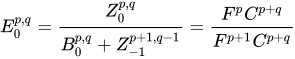
$E_{0}^{p,q}={\frac {Z_{0}^{p,q}}{B_{0}^{p,q}+Z_{-1}^{p+1,q-1}}}={\frac {F^{p}C^{p+q}}{F^{p+1}C^{p+q}}}$

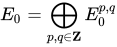
$E_{0}=\bigoplus _{p,q\in \mathbf {Z} }E_{0}^{p,q}$

Since we assumed that the boundary map was compatible with the filtration, $E_{0}$ is a doubly graded object and there is a natural doubly graded boundary map $d_{0}$ on $E_{0}$ . To get $E_{1}$ , we take the homology of $E_{0}$ .

${\bar {Z}}_{1}^{p,q}=\ker d_{0}^{p,q}:E_{0}^{p,q}\rightarrow E_{0}^{p,q+1}=\ker d_{0}^{p,q}:F^{p}C^{p+q}/F^{p+1}C^{p+q}\rightarrow F^{p}C^{p+q+1}/F^{p+1}C^{p+q+1}$

${\bar {B}}_{1}^{p,q}={\mbox{im }}d_{0}^{p,q-1}:E_{0}^{p,q-1}\rightarrow E_{0}^{p,q}={\mbox{im }}d_{0}^{p,q-1}:F^{p}C^{p+q-1}/F^{p+1}C^{p+q-1}\rightarrow F^{p}C^{p+q}/F^{p+1}C^{p+q}$

$E_{1}^{p,q}={\frac {{\bar {Z}}_{1}^{p,q}}{{\bar {B}}_{1}^{p,q}}}={\frac {\ker d_{0}^{p,q}:E_{0}^{p,q}\rightarrow E_{0}^{p,q+1}}{{\mbox{im }}d_{0}^{p,q-1}:E_{0}^{p,q-1}\rightarrow E_{0}^{p,q}}}$

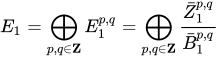
$E_{1}=\bigoplus _{p,q\in \mathbf {Z} }E_{1}^{p,q}=\bigoplus _{p,q\in \mathbf {Z} }{\frac {{\bar {Z}}_{1}^{p,q}}{{\bar {B}}_{1}^{p,q}}}$

Notice that ${\bar {Z}}_{1}^{p,q}$ and ${\bar {B}}_{1}^{p,q}$ can be written as the images in $E_{0}^{p,q}$ of

$Z_{1}^{p,q}=\ker d_{0}^{p,q}:F^{p}C^{p+q}\rightarrow C^{p+q+1}/F^{p+1}C^{p+q+1}$

$B_{1}^{p,q}=({\mbox{im }}d_{0}^{p,q-1}:F^{p}C^{p+q-1}\rightarrow C^{p+q})\cap F^{p}C^{p+q}$

and that we then have

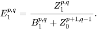
$E_{1}^{p,q}={\frac {Z_{1}^{p,q}}{B_{1}^{p,q}+Z_{0}^{p+1,q-1}}}.$

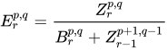
$Z_{1}^{p,q}$ are exactly the elements which the differential pushes up one level in the filtration, and $B_{1}^{p,q}$ are exactly the image of the elements which the differential pushes up zero levels in the filtration. This suggests that we should choose $Z_{r}^{p,q}$ to be the elements which the differential pushes up r levels in the filtration and $B_{r}^{p,q}$ to be image of the elements which the differential pushes up r-1 levels in the filtration. In other words, the spectral sequence should satisfy

$Z_{r}^{p,q}=\ker d_{0}^{p,q}:F^{p}C^{p+q}\rightarrow C^{p+q+1}/F^{p+r}C^{p+q+1}$

$B_{r}^{p,q}=({\mbox{im }}d_{0}^{p-r+1,q+r-2}:F^{p-r+1}C^{p+q-1}\rightarrow C^{p+q})\cap F^{p}C^{p+q}$

$E_{r}^{p,q}={\frac {Z_{r}^{p,q}}{B_{r}^{p,q}+Z_{r-1}^{p+1,q-1}}}$

and we should have the relationship

$B_{r}^{p,q}=d_{0}^{p,q}(Z_{r-1}^{p-r+1,q+r-2}).$

For this to make sense, we must find a differential $d_{r}$ on each $E_{r}$ and verify that it leads to homology isomorphic to $E_{r+1}$ . The differential

$d_{r}^{p,q}:E_{r}^{p,q}\rightarrow E_{r}^{p+r,q-r+1}$

is defined by restricting the original differential $d$ defined on $C^{p+q}$ to the subobject $Z_{r}^{p,q}$ . It is straightforward to check that the homology of $E_{r}$ with respect to this differential is $E_{r+1}$ , so this gives a spectral sequence. Unfortunately, the differential is not very explicit. Determining differentials or finding ways to work around them is one of the main challenges to successfully applying a spectral sequence.

Spectral sequences constructed with this method

Hodge-de Rham spectral sequence
Spectral sequence of a double complex
Can be used to construct Mixed Hodge structures

The spectral sequence of a double complex

Another common spectral sequence is the spectral sequence of a double complex. A double complex is a collection of objects C_i,j for all integers i and j together with two differentials, d^I and d^II. d^I is assumed to decrease i, and d^II is assumed to decrease j. Furthermore, we assume that the differentials anticommute, so that d^I d^II + d^II d^I = 0. Our goal is to compare the iterated homologies $H_{i}^{\textrm {I}}(H_{j}^{\textrm {II}}(C_{\bullet ,\bullet }))$ and $H_{j}^{\textrm {II}}(H_{i}^{\textrm {I}}(C_{\bullet ,\bullet }))$ . We will do this by filtering our double complex in two different ways. Here are our filtrations:

$(C_{i,j}^{\textrm {I}})_{p}={\begin{cases}0&{\text{if }}i<p\\C_{i,j}&{\text{if }}i\geq p\end{cases}}$

$(C_{i,j}^{\textrm {II}})_{p}={\begin{cases}0&{\text{if }}j<p\\C_{i,j}&{\text{if }}j\geq p\end{cases}}$

To get a spectral sequence, we will reduce to the previous example. We define the total complex T(C_•,•) to be the complex whose n′th term is $\bigoplus _{i+j=n}C_{i,j}$ and whose differential is d^I + d^II. This is a complex because d^I and d^II are anticommuting differentials. The two filtrations on C_i,j give two filtrations on the total complex:

$T_{n}(C_{\bullet ,\bullet })_{p}^{\textrm {I}}=\bigoplus _{i+j=n \atop i>p-1}C_{i,j}$

$T_{n}(C_{\bullet ,\bullet })_{p}^{\textrm {II}}=\bigoplus _{i+j=n \atop j>p-1}C_{i,j}$

To show that these spectral sequences give information about the iterated homologies, we will work out the E⁰, E¹, and E² terms of the I filtration on T(C_•,•). The E⁰ term is clear:

${}^{\textrm {I}}E_{p,q}^{0}=T_{n}(C_{\bullet ,\bullet })_{p}^{\textrm {I}}/T_{n}(C_{\bullet ,\bullet })_{p+1}^{\textrm {I}}=\bigoplus _{i+j=n \atop i>p-1}C_{i,j}{\Big /}\bigoplus _{i+j=n \atop i>p}C_{i,j}=C_{p,q},$

where n = p + q.

To find the E¹ term, we need to determine d^I + d^II on E⁰. Notice that the differential must have degree −1 with respect to n, so we get a map

$d_{p,q}^{\textrm {I}}+d_{p,q}^{\textrm {II}}:T_{n}(C_{\bullet ,\bullet })_{p}^{\textrm {I}}/T_{n}(C_{\bullet ,\bullet })_{p+1}^{\textrm {I}}=C_{p,q}\rightarrow T_{n-1}(C_{\bullet ,\bullet })_{p}^{\textrm {I}}/T_{n-1}(C_{\bullet ,\bullet })_{p+1}^{\textrm {I}}=C_{p,q-1}$

Consequently, the differential on E⁰ is the map C_p,q → C_p,q−1 induced by d^I + d^II. But d^I has the wrong degree to induce such a map, so d^I must be zero on E⁰. That means the differential is exactly d^II, so we get

${}^{\textrm {I}}E_{p,q}^{1}=H_{q}^{\textrm {II}}(C_{p,\bullet }).$

To find E², we need to determine

$d_{p,q}^{\textrm {I}}+d_{p,q}^{\textrm {II}}:H_{q}^{\textrm {II}}(C_{p,\bullet })\rightarrow H_{q}^{\textrm {II}}(C_{p+1,\bullet })$

Because E¹ was exactly the homology with respect to d^II, d^II is zero on E¹. Consequently, we get

${}^{\textrm {I}}E_{p,q}^{2}=H_{p}^{\textrm {I}}(H_{q}^{\textrm {II}}(C_{\bullet ,\bullet })).$

Using the other filtration gives us a different spectral sequence with a similar E² term:

${}^{\textrm {II}}E_{p,q}^{2}=H_{q}^{\textrm {II}}(H_{p}^{I}(C_{\bullet ,\bullet })).$

What remains is to find a relationship between these two spectral sequences. It will turn out that as r increases, the two sequences will become similar enough to allow useful comparisons.

06Convergence, degeneration, and abutment

Interpretation as a filtration of cycles and boundaries

Let E_r be a spectral sequence, starting with say r = 1. Then there is a sequence of subobjects

$0=B_{0}\subset B_{1}\subset B_{2}\subset \dots \subset B_{r}\subset \dots \subset Z_{r}\subset \dots \subset Z_{2}\subset Z_{1}\subset Z_{0}=E_{1}$

such that $E_{r}\simeq Z_{r-1}/B_{r-1}$ ; indeed, recursively we let $Z_{0}=E_{1},B_{0}=0$ and let $Z_{r},B_{r}$ be so that $Z_{r}/B_{r-1},B_{r}/B_{r-1}$ are the kernel and the image of $E_{r}{\overset {d_{r}}{\to }}E_{r}.$

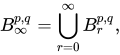
We then let $\textstyle Z_{\infty }=\bigcap _{r}Z_{r},B_{\infty }=\bigcup _{r}B_{r}$ and

$E_{\infty }=Z_{\infty }/B_{\infty }$ ;

it is called the limiting term. (Of course, such $E_{\infty }$ need not exist in the category, but this is usually a non-issue since for example in the category of modules such limits exist or since in practice a spectral sequence one works with tends to degenerate; there are only finitely many inclusions in the sequence above.)

Terms of convergence

We say a spectral sequence converges weakly if there is a graded object $H^{\bullet }$ with a filtration $F^{\bullet }H^{n}$ for every $n$ , and for every $p$ there exists an isomorphism $E_{\infty }^{p,q}\cong F^{p}H^{p+q}/F^{p+1}H^{p+q}$ . It converges to $H^{\bullet }$ if the filtration $F^{\bullet }H^{n}$ is Hausdorff, i.e. $\textstyle \bigcap _{p}F^{p}H^{\bullet }=0$ . We write

$E_{r}^{p,q}\Rightarrow _{p}E_{\infty }^{n}$

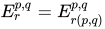
to mean that whenever p + q = n, $E_{r}^{p,q}$ converges to $E_{\infty }^{p,q}$ . We say that a spectral sequence $E_{r}^{p,q}$ abuts to $E_{\infty }^{p,q}$ (the spectral sequence abutment) if for every $p,q$ there is $r(p,q)$ such that for all $r\geq r(p,q)$ , $E_{r}^{p,q}=E_{r(p,q)}^{p,q}$ . Then $E_{r(p,q)}^{p,q}=E_{\infty }^{p,q}$ is the limiting term. The spectral sequence is regular or degenerates at $r_{0}$ if the differentials $d_{r}^{p,q}$ are zero for all $r\geq r_{0}$ . If in particular there is $r_{0}\geq 2$ , such that the $r_{0}^{th}$ sheet is concentrated on a single row or a single column, then we say it collapses. In symbols, we write:

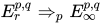
$E_{r}^{p,q}\Rightarrow _{p}E_{\infty }^{p,q}$

The p indicates the filtration index. It is very common to write the $E_{2}^{p,q}$ term on the left-hand side of the abutment, because this is the most useful term of most spectral sequences. The spectral sequence of an unfiltered chain complex degenerates at the first sheet (see first example): since nothing happens after the zeroth sheet, the limiting sheet $E_{\infty }$ is the same as $E_{1}$ .

The five-term exact sequence of a spectral sequence relates certain low-degree terms and E_∞ terms.

07Examples of degeneration

The spectral sequence of a filtered complex, continued

Notice that we have a chain of inclusions:

$Z_{0}^{p,q}\supseteq Z_{1}^{p,q}\supseteq Z_{2}^{p,q}\supseteq \cdots \supseteq B_{2}^{p,q}\supseteq B_{1}^{p,q}\supseteq B_{0}^{p,q}$

We can ask what happens if we define

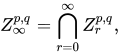
$Z_{\infty }^{p,q}=\bigcap _{r=0}^{\infty }Z_{r}^{p,q},$

$B_{\infty }^{p,q}=\bigcup _{r=0}^{\infty }B_{r}^{p,q},$

$E_{\infty }^{p,q}={\frac {Z_{\infty }^{p,q}}{B_{\infty }^{p,q}+Z_{\infty }^{p+1,q-1}}}.$

$E_{\infty }^{p,q}$ is a natural candidate for the abutment of this spectral sequence. Convergence is not automatic, but happens in many cases. In particular, if the filtration is finite and consists of exactly r nontrivial steps, then the spectral sequence degenerates after the rth sheet. Convergence also occurs if the complex and the filtration are both bounded below or both bounded above.

To describe the abutment of our spectral sequence in more detail, notice that we have the formulas:

$Z_{\infty }^{p,q}=\bigcap _{r=0}^{\infty }Z_{r}^{p,q}=\bigcap _{r=0}^{\infty }\ker(F^{p}C^{p+q}\rightarrow C^{p+q+1}/F^{p+r}C^{p+q+1})$

$B_{\infty }^{p,q}=\bigcup _{r=0}^{\infty }B_{r}^{p,q}=\bigcup _{r=0}^{\infty }({\mbox{im }}d^{p,q-r}:F^{p-r}C^{p+q-1}\rightarrow C^{p+q})\cap F^{p}C^{p+q}$

To see what this implies for $Z_{\infty }^{p,q}$ recall that we assumed that the filtration was separated. This implies that as r increases, the kernels shrink, until we are left with $Z_{\infty }^{p,q}=\ker(F^{p}C^{p+q}\rightarrow C^{p+q+1})$ . For $B_{\infty }^{p,q}$ , recall that we assumed that the filtration was exhaustive. This implies that as r increases, the images grow until we reach $B_{\infty }^{p,q}={\text{im }}(C^{p+q-1}\rightarrow C^{p+q})\cap F^{p}C^{p+q}$ . We conclude

$E_{\infty }^{p,q}={\mbox{gr}}_{p}H^{p+q}(C^{\bullet })$ ,

that is, the abutment of the spectral sequence is the pth graded part of the (p+q)th homology of C. If our spectral sequence converges, then we conclude that:

$E_{r}^{p,q}\Rightarrow _{p}H^{p+q}(C^{\bullet })$

Long exact sequences

Using the spectral sequence of a filtered complex, we can derive the existence of long exact sequences. Choose a short exact sequence of cochain complexes 0 → A^• → B^• → C^• → 0, and call the first map f^• : A^• → B^•. We get natural maps of homology objects Hⁿ(A^•) → Hⁿ(B^•) → Hⁿ(C^•), and we know that this is exact in the middle. We will use the spectral sequence of a filtered complex to find the connecting homomorphism and to prove that the resulting sequence is exact.To start, we filter B^•:

$F^{0}B^{n}=B^{n}$

$F^{1}B^{n}=A^{n}$

$F^{2}B^{n}=0$

This gives:

$E_{0}^{p,q}={\frac {F^{p}B^{p+q}}{F^{p+1}B^{p+q}}}={\begin{cases}0&{\text{if }}p<0{\text{ or }}p>1\\C^{q}&{\text{if }}p=0\\A^{q+1}&{\text{if }}p=1\end{cases}}$

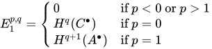
$E_{1}^{p,q}={\begin{cases}0&{\text{if }}p<0{\text{ or }}p>1\\H^{q}(C^{\bullet })&{\text{if }}p=0\\H^{q+1}(A^{\bullet })&{\text{if }}p=1\end{cases}}$

The differential has bidegree (1, 0), so d_0,q : H^q(C^•) → H^q+1(A^•). These are the connecting homomorphisms from the snake lemma, and together with the maps A^• → B^• → C^•, they give a sequence:

$\cdots \rightarrow H^{q}(B^{\bullet })\rightarrow H^{q}(C^{\bullet })\rightarrow H^{q+1}(A^{\bullet })\rightarrow H^{q+1}(B^{\bullet })\rightarrow \cdots$

It remains to show that this sequence is exact at the A and C spots. Notice that this spectral sequence degenerates at the E₂ term because the differentials have bidegree (2, −1). Consequently, the E₂ term is the same as the E_∞ term:

$E_{2}^{p,q}\cong {\text{gr}}_{p}H^{p+q}(B^{\bullet })={\begin{cases}0&{\text{if }}p<0{\text{ or }}p>1\\H^{q}(B^{\bullet })/H^{q}(A^{\bullet })&{\text{if }}p=0\\{\text{im }}H^{q+1}f^{\bullet }:H^{q+1}(A^{\bullet })\rightarrow H^{q+1}(B^{\bullet })&{\text{if }}p=1\end{cases}}$

But we also have a direct description of the E₂ term as the homology of the E₁ term. These two descriptions must be isomorphic:

$H^{q}(B^{\bullet })/H^{q}(A^{\bullet })\cong \ker d_{0,q}^{1}:H^{q}(C^{\bullet })\rightarrow H^{q+1}(A^{\bullet })$

${\text{im }}H^{q+1}f^{\bullet }:H^{q+1}(A^{\bullet })\rightarrow H^{q+1}(B^{\bullet })\cong H^{q+1}(A^{\bullet })/({\mbox{im }}d_{0,q}^{1}:H^{q}(C^{\bullet })\rightarrow H^{q+1}(A^{\bullet }))$

The former gives exactness at the C spot, and the latter gives exactness at the A spot.

The spectral sequence of a double complex, continued

Using the abutment for a filtered complex, we find that:

$H_{p}^{\textrm {I}}(H_{q}^{\textrm {II}}(C_{\bullet ,\bullet }))\Rightarrow _{p}H^{p+q}(T(C_{\bullet ,\bullet }))$

$H_{q}^{\textrm {II}}(H_{p}^{\textrm {I}}(C_{\bullet ,\bullet }))\Rightarrow _{q}H^{p+q}(T(C_{\bullet ,\bullet }))$

In general, the two gradings on ⁠ $H^{p+q}(T(C_{\bullet ,\bullet }))$ ⁠ are distinct. Despite this, it is still possible to gain useful information from these two spectral sequences.

Commutativity of Tor

Let R be a ring, let M be a right R-module and N a left R-module. Recall that the derived functors of the tensor product are denoted Tor. Tor is defined using a projective resolution of its first argument. However, it turns out that $\operatorname {Tor} _{i}(M,N)=\operatorname {Tor} _{i}(N,M)$ . While this can be verified without a spectral sequence, it is very easy with spectral sequences.

Choose projective resolutions $P_{\bullet }$ and $Q_{\bullet }$ of M and N, respectively. Consider these as complexes which vanish in negative degree having differentials d and e, respectively. We can construct a double complex whose terms are $C_{i,j}=P_{i}\otimes Q_{j}$ and whose differentials are $d\otimes 1$ and $(-1)^{\textrm {I}}(1\otimes e)$ . (The factor of −1 is so that the differentials anticommute.) Since projective modules are flat, taking the tensor product with a projective module commutes with taking homology, so we get:

$H_{p}^{\textrm {I}}(H_{q}^{\textrm {II}}(P_{\bullet }\otimes Q_{\bullet }))=H_{p}^{\textrm {I}}(P_{\bullet }\otimes H_{q}^{\textrm {II}}(Q_{\bullet }))$

$H_{q}^{\textrm {II}}(H_{p}^{\textrm {I}}(P_{\bullet }\otimes Q_{\bullet }))=H_{q}^{\textrm {II}}(H_{p}^{\textrm {I}}(P_{\bullet })\otimes Q_{\bullet })$

Since the two complexes are resolutions, their homology vanishes outside of degree zero. In degree zero, we are left with

$H_{p}^{\textrm {I}}(P_{\bullet }\otimes N)=\operatorname {Tor} _{p}(M,N)$

$H_{q}^{\textrm {II}}(M\otimes Q_{\bullet })=\operatorname {Tor} _{q}(N,M)$

In particular, the $E_{p,q}^{2}$ terms vanish except along the lines q = 0 (for the I spectral sequence) and p = 0 (for the II spectral sequence). This implies that the spectral sequence degenerates at the second sheet, so the E^∞ terms are isomorphic to the E² terms:

$\operatorname {Tor} _{p}(M,N)\cong E_{p}^{\infty }=H_{p}(T(C_{\bullet ,\bullet }))$

$\operatorname {Tor} _{q}(N,M)\cong E_{q}^{\infty }=H_{q}(T(C_{\bullet ,\bullet }))$

Finally, when p and q are equal, the two right-hand sides are equal, and the commutativity of Tor follows.

08Worked-out examples

First-quadrant sheet

Consider a spectral sequence where $E_{r}^{p,q}$ vanishes for all $p$ less than some $p_{0}$ and for all $q$ less than some $q_{0}$ . If $p_{0}$ and $q_{0}$ can be chosen to be zero, this is called a first-quadrant spectral sequence. The sequence abuts because $E_{r+i}^{p,q}=E_{r}^{p,q}$ holds for all $i\geq 0$ if $r>p$ and $r>q+1$ . To see this, note that either the domain or the codomain of the differential is zero for the considered cases. In visual terms, the sheets stabilize in a growing rectangle (see picture above). The spectral sequence need not degenerate, however, because the differential maps might not all be zero at once. Similarly, the spectral sequence also converges if $E_{r}^{p,q}$ vanishes for all $p$ greater than some $p_{0}$ and for all $q$ greater than some $q_{0}$ .

2 non-zero adjacent columns

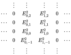
Let $E_{p,q}^{r}$ be a homological spectral sequence such that $E_{p,q}^{2}=0$ for all p other than 0, 1. Visually, this is the spectral sequence with $E^{2}$ -page

${\begin{matrix}&\vdots &\vdots &\vdots &\vdots &\\\cdots &0&E_{0,2}^{2}&E_{1,2}^{2}&0&\cdots \\\cdots &0&E_{0,1}^{2}&E_{1,1}^{2}&0&\cdots \\\cdots &0&E_{0,0}^{2}&E_{1,0}^{2}&0&\cdots \\\cdots &0&E_{0,-1}^{2}&E_{1,-1}^{2}&0&\cdots \\&\vdots &\vdots &\vdots &\vdots &\end{matrix}}$

The differentials on the second page have degree (-2, 1), so they are of the form

$d_{p,q}^{2}:E_{p,q}^{2}\to E_{p-2,q+1}^{2}$

These maps are all zero since they are

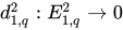
$d_{0,q}^{2}:E_{0,q}^{2}\to 0$ , $d_{1,q}^{2}:E_{1,q}^{2}\to 0$

hence the spectral sequence degenerates: $E^{\infty }=E^{2}$ . Say, it converges to $H_{*}$ with a filtration

$0=F_{-1}H_{n}\subset F_{0}H_{n}\subset \dots \subset F_{n}H_{n}=H_{n}$

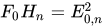
such that $E_{p,q}^{\infty }=F_{p}H_{p+q}/F_{p-1}H_{p+q}$ . Then $F_{0}H_{n}=E_{0,n}^{2}$ , $F_{1}H_{n}/F_{0}H_{n}=E_{1,n-1}^{2}$ , $F_{2}H_{n}/F_{1}H_{n}=0$ , $F_{3}H_{n}/F_{2}H_{n}=0$ , etc. Thus, there is the exact sequence:

$0\to E_{0,n}^{2}\to H_{n}\to E_{1,n-1}^{2}\to 0$ .

Next, let $E_{p,q}^{r}$ be a spectral sequence whose second page consists only of two lines q = 0, 1. This need not degenerate at the second page but it still degenerates at the third page as the differentials there have degree (-3, 2). Note $E_{p,0}^{3}=\operatorname {ker} (d:E_{p,0}^{2}\to E_{p-2,1}^{2})$ , as the denominator is zero. Similarly, $E_{p,1}^{3}=\operatorname {coker} (d:E_{p+2,0}^{2}\to E_{p,1}^{2})$ . Thus,

$0\to E_{p,0}^{\infty }\to E_{p,0}^{2}{\overset {d}{\to }}E_{p-2,1}^{2}\to E_{p-2,1}^{\infty }\to 0$ .

Now, say, the spectral sequence converges to H with a filtration F as in the previous example. Since $F_{p-2}H_{p}/F_{p-3}H_{p}=E_{p-2,2}^{\infty }=0$ , $F_{p-3}H_{p}/F_{p-4}H_{p}=0$ , etc., we have: $0\to E_{p-1,1}^{\infty }\to H_{p}\to E_{p,0}^{\infty }\to 0$ . Putting everything together, one gets:

$\cdots \to H_{p+1}\to E_{p+1,0}^{2}{\overset {d}{\to }}E_{p-1,1}^{2}\to H_{p}\to E_{p,0}^{2}{\overset {d}{\to }}E_{p-2,1}^{2}\to H_{p-1}\to \dots .$

Wang sequence

The computation in the previous section generalizes in a straightforward way. Consider a fibration over a sphere:

$F{\overset {i}{\to }}E{\overset {p}{\to }}S^{n}$

with n at least 2. There is the Serre spectral sequence:

$E_{p,q}^{2}=H_{p}(S^{n};H_{q}(F))\Rightarrow H_{p+q}(E)$ ;

that is to say, $E_{p,q}^{\infty }=F_{p}H_{p+q}(E)/F_{p-1}H_{p+q}(E)$ with some filtration $F_{\bullet }$ .

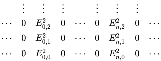
Since $H_{p}(S^{n})$ is nonzero only when p is zero or n and equal to Z in that case, we see $E_{p,q}^{2}$ consists of only two lines $p=0,n$ , hence the $E^{2}$ -page is given by

${\begin{matrix}&\vdots &\vdots &\vdots &&\vdots &\vdots &\vdots &\\\cdots &0&E_{0,2}^{2}&0&\cdots &0&E_{n,2}^{2}&0&\cdots \\\cdots &0&E_{0,1}^{2}&0&\cdots &0&E_{n,1}^{2}&0&\cdots \\\cdots &0&E_{0,0}^{2}&0&\cdots &0&E_{n,0}^{2}&0&\cdots \\\end{matrix}}$

Moreover, since

$E_{p,q}^{2}=H_{p}(S^{n};H_{q}(F))=H_{q}(F)$

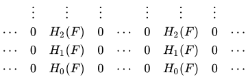
for $p=0,n$ by the universal coefficient theorem, the $E^{2}$ page looks like

${\begin{matrix}&\vdots &\vdots &\vdots &&\vdots &\vdots &\vdots &\\\cdots &0&H_{2}(F)&0&\cdots &0&H_{2}(F)&0&\cdots \\\cdots &0&H_{1}(F)&0&\cdots &0&H_{1}(F)&0&\cdots \\\cdots &0&H_{0}(F)&0&\cdots &0&H_{0}(F)&0&\cdots \\\end{matrix}}$

Since the only non-zero differentials are on the $E^{n}$ -page, given by

$d_{n,q}^{n}:E_{n,q}^{n}\to E_{0,q+n-1}^{n}$

which is

$d_{n,q}^{n}:H_{q}(F)\to H_{q+n-1}(F)$

the spectral sequence converges on $E^{n+1}=E^{\infty }$ . By computing $E^{n+1}$ we get an exact sequence

$0\to E_{n,q-n}^{\infty }\to E_{n,q-n}^{n}{\overset {d}{\to }}E_{0,q-1}^{n}\to E_{0,q-1}^{\infty }\to 0.$

and written out using the homology groups, this is

$0\to E_{n,q-n}^{\infty }\to H_{q-n}(F){\overset {d}{\to }}H_{q-1}(F)\to E_{0,q-1}^{\infty }\to 0.$

To establish what the two $E^{\infty }$ -terms are, write $H=H(E)$ , and since $F_{1}H_{q}/F_{0}H_{q}=E_{1,q-1}^{\infty }=0$ , etc., we have: $E_{n,q-n}^{\infty }=F_{n}H_{q}/F_{0}H_{q}$ and thus, since $F_{0}H_{q}=E_{0,q}^{\infty }$ and $F_{n}H_{q}=H_{q}$ as the first and the last term of the filtration,

$0\to E_{0,q}^{\infty }\to H_{q}\to E_{n,q-n}^{\infty }\to 0.$

This is the exact sequence

$0\to H_{q}(F)\to H_{q}(E)\to H_{q-n}(F)\to 0.$

Putting all calculations together, one gets:

$\dots \to H_{q}(F){\overset {i_{*}}{\to }}H_{q}(E)\to H_{q-n}(F){\overset {d}{\to }}H_{q-1}(F){\overset {i_{*}}{\to }}H_{q-1}(E)\to H_{q-n-1}(F)\to \dots$

(The Gysin sequence is obtained in a similar way.)

Low-degree terms

With an obvious notational change, the type of the computations in the previous examples can also be carried out for cohomological spectral sequence. Let $E_{r}^{p,q}$ be a first-quadrant spectral sequence converging to H with the decreasing filtration

$0=F^{n+1}H^{n}\subset F^{n}H^{n}\subset \dots \subset F^{0}H^{n}=H^{n}$

so that $E_{\infty }^{p,q}=F^{p}H^{p+q}/F^{p+1}H^{p+q}.$ Since $E_{2}^{p,q}$ is zero if p or q is negative, we have:

$0\to E_{\infty }^{0,1}\to E_{2}^{0,1}{\overset {d}{\to }}E_{2}^{2,0}\to E_{\infty }^{2,0}\to 0.$

Since $E_{\infty }^{1,0}=E_{2}^{1,0}$ for the same reason and since $F^{2}H^{1}=0,$

$0\to E_{2}^{1,0}\to H^{1}\to E_{\infty }^{0,1}\to 0$ .

Since $F^{3}H^{2}=0$ , $E_{\infty }^{2,0}\subset H^{2}$ . Stacking the sequences together, we get the so-called five-term exact sequence:

$0\to E_{2}^{1,0}\to H^{1}\to E_{2}^{0,1}{\overset {d}{\to }}E_{2}^{2,0}\to H^{2}.$

09Edge maps and transgressions

Homological spectral sequences

Let $E_{p,q}^{r}$ be a spectral sequence. If $E_{p,q}^{r}=0$ for every q < 0, then it must be that: for r ≥ 2,

$E_{p,0}^{r+1}=\operatorname {ker} (d:E_{p,0}^{r}\to E_{p-r,r-1}^{r})$

as the denominator is zero. Hence, there is a sequence of monomorphisms:

$E_{p,0}^{r}\to E_{p,0}^{r-1}\to \dots \to E_{p,0}^{3}\to E_{p,0}^{2}$ .

They are called the edge maps. Similarly, if $E_{p,q}^{r}=0$ for every p < 0, then there is a sequence of epimorphisms (also called the edge maps):

$E_{0,q}^{2}\to E_{0,q}^{3}\to \dots \to E_{0,q}^{r-1}\to E_{0,q}^{r}$ .

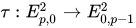
The transgression is a partially defined map (more precisely, a map from a subobject to a quotient)

$\tau :E_{p,0}^{2}\to E_{0,p-1}^{2}$

given as a composition $E_{p,0}^{2}\to E_{p,0}^{p}{\overset {d}{\to }}E_{0,p-1}^{p}\to E_{0,p-1}^{2}$ , the first and last maps being the inverses of the edge maps.

Cohomological spectral sequences

For a spectral sequence $E_{r}^{p,q}$ of cohomological type, the analogous statements hold. If $E_{r}^{p,q}=0$ for every q < 0, then there is a sequence of epimorphisms

$E_{2}^{p,0}\to E_{3}^{p,0}\to \dots \to E_{r-1}^{p,0}\to E_{r}^{p,0}$ .

And if $E_{r}^{p,q}=0$ for every p < 0, then there is a sequence of monomorphisms:

$E_{r}^{0,q}\to E_{r-1}^{0,q}\to \dots \to E_{3}^{0,q}\to E_{2}^{0,q}$ .

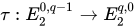
The transgression is a not necessarily well-defined map:

$\tau :E_{2}^{0,q-1}\to E_{2}^{q,0}$

induced by $d:E_{q}^{0,q-1}\to E_{q}^{q,0}$ .

Application

Determining these maps are fundamental for computing many differentials in the Serre spectral sequence. For instance the transgression map determines the differential

$d_{n}:E_{n,0}^{n}\to E_{0,n-1}^{n}$

for the homological spectral spectral sequence, hence on the Serre spectral sequence for a fibration $F\to E\to B$ gives the map

$d_{n}:H_{n}(B)\to H_{n-1}(F)$ .

10Further examples

Some notable spectral sequences are:

Topology and geometry

Atiyah-Hirzebruch spectral sequence of an extraordinary cohomology theory
Bar spectral sequence for the homology of the classifying space of a group.
Bockstein spectral sequence relating the homology with mod p coefficients and the homology reduced mod p.
Cartan-Leray spectral sequence converging to the homology of a quotient space.
Eilenberg-Moore spectral sequence for the singular cohomology of the pullback of a fibration
Serre spectral sequence of a fibration

Homotopy theory

Adams spectral sequence in stable homotopy theory
Adams-Novikov spectral sequence, a generalization to extraordinary cohomology theories.
Barratt spectral sequence converging to the homotopy of the initial space of a cofibration.
Bousfield-Kan spectral sequence converging to the homotopy colimit of a functor.
Chromatic spectral sequence for calculating the initial terms of the Adams-Novikov spectral sequence.
Cobar spectral sequence
EHP spectral sequence converging to stable homotopy groups of spheres
Federer spectral sequence converging to homotopy groups of a function space.
Homotopy fixed point spectral sequence
Hurewicz spectral sequence for calculating the homology of a space from its homotopy.
Miller spectral sequence converging to the mod p stable homology of a space.
Milnor spectral sequence is another name for the bar spectral sequence.
Moore spectral sequence is another name for the bar spectral sequence.
Quillen spectral sequence for calculating the homotopy of a simplicial group.
Rothenberg-Steenrod spectral sequence is another name for the bar spectral sequence.
van Kampen spectral sequence for calculating the homotopy of a wedge of spaces.

Algebra

Čech-to-derived functor spectral sequence from Čech cohomology to sheaf cohomology.
Change of rings spectral sequences for calculating Tor and Ext groups of modules.
Connes spectral sequences converging to the cyclic homology of an algebra.
Gersten-Witt spectral sequence
Green's spectral sequence for Koszul cohomology
Grothendieck spectral sequence for composing derived functors
Hyperhomology spectral sequence for calculating hyperhomology.
Künneth spectral sequence for calculating the homology of a tensor product of differential algebras.
Leray spectral sequence converging to the cohomology of a sheaf.
Local-to-global Ext spectral sequence
Lyndon-Hochschild-Serre spectral sequence in group (co)homology
May spectral sequence for calculating the Tor or Ext groups of an algebra.
Spectral sequence of a differential filtered group: described in this article.
Spectral sequence of a double complex: described in this article.
Spectral sequence of an exact couple: described in this article.
Universal coefficient spectral sequence
van Est spectral sequence converging to relative Lie algebra cohomology.

Complex and algebraic geometry

Arnold's spectral sequence in singularity theory.
Bloch-Lichtenbaum spectral sequence converging to the algebraic K-theory of a field.
Frölicher spectral sequence starting from the Dolbeault cohomology and converging to the algebraic de Rham cohomology of a variety.
Hodge-de Rham spectral sequence converging to the algebraic de Rham cohomology of a variety.
Motivic-to-K-theory spectral sequence

Watch videos about Spectral sequenceExplainers and documentaries on YouTube (opens in a new tab)

Sources and credits

This article is adapted from the Wikipedia article “Spectral sequence”, written by its contributors and licensed under CC BY-SA 4.0. Fathomly has changed the layout, removed citation markers, navigation and maintenance notices, and adjusted punctuation. This adapted version is shared under the same license. For references, see the original article.

Images, from Wikimedia Commons:

SpectralSequence.png by Saaska at English Wikipedia, Public domain
Spectral Sequence Visualization.jpg by L.penguu, CC BY-SA 4.0
Exact couple.png by Jakob.scholbach at English Wikipedia, CC BY-SA 3.0

Fathomly is not affiliated with or endorsed by the Wikimedia Foundation. Spotted a problem? Tell us.