Encyclopedia

Source field

Type of field appearing in the Lagrangian

Wikipedia contributorsAdapted for Fathomly · View authors

9 min read
Source updated September 14, 2026

In theoretical physics, a source is an abstract concept, developed by Julian Schwinger, motivated by the physical effects of surrounding particles involved in creating or destroying another particle. So, one can perceive sources as the origin of the physical properties carried by the created or destroyed particle, and thus one can use this concept to study all quantum processes including the spacetime localized properties and the energy forms, i.e., mass and momentum, of the phenomena. The probability amplitude of the created or the decaying particle is defined by the effect of the source on a localized spacetime region such that the affected particle captures its physics depending on the tensorial and spinorial nature of the source. An example that Julian Schwinger referred to is the creation of $\eta ^{*}$ meson due to the mass correlations among five $\pi$ mesons.

The same idea can be used to define source fields. Mathematically, a source field is a background field $J$ coupled to the original field $\phi$ as $S_{\text{source}}=J\phi .$ This term appears in the action in Richard Feynman's path integral formulation and is responsible for the theory interactions. In a collision reaction a source could be other particles in the collision. Therefore, the source appears in the vacuum amplitude acting from both sides on the Green's function correlator of the theory.

Schwinger's source theory stems from Schwinger's quantum action principle and can be related to the path integral formulation as the variation with respect to the source per se $\delta J$ corresponds to the field $\phi$ , i.e.

$\delta J=\int {\mathcal {D}}\phi \,\exp \left(-i\!\int \!d^{4}x\,J(x,t)\phi (x,t)\right).$

Also, a source acts effectively in a region of the spacetime. As one sees in the examples below, the source field appears on the right-hand side of the equations of motion (usually second-order partial differential equations) for $\phi$ . When the field $\phi$ is the electromagnetic potential or the metric tensor, the source field is the electric current or the stress-energy tensor, respectively.

In terms of the statistical and non-relativistic applications, Schwinger's source formulation plays crucial rules in understanding many non-equilibrium systems. Source theory is theoretically significant as it needs neither divergence regularizations nor renormalization.

01Relation between path integral formulation and source formulation

In the Feynman's path integral formulation with normalization ${\mathcal {N}}\equiv Z[J=0]$ , the partition function is given by

$Z[J]={\mathcal {N}}\int {\mathcal {D}}\phi \,\exp \left[-i\left(\int dt~{\mathcal {L}}(t;\phi ,{\dot {\phi }})+\int d^{4}x\,J(x,t)\phi (x,t)\right)\right].$

One can expand the current term in the exponent ${\mathcal {N}}\int {\mathcal {D}}\phi ~\exp \left(-i\int d^{4}x\,J(x,t)\phi (x,t)\right)={\mathcal {N}}\sum _{n=0}^{\infty }{\frac {i^{n}}{n!}}\int d^{4}x_{1}\cdots \int d^{4}x_{n}J(x_{1})\cdots J(x_{1})\left\langle \phi (x_{1})\cdots \phi (x_{n})\right\rangle$

to generate Green's functions (correlators) $G(t_{1},\cdots ,t_{n})={\left(-i\right)}^{n}\left.{\frac {\delta ^{n}Z[J]}{\delta J(t_{1})\cdots \delta J(t_{n})}}\right|_{J=0},$ where the fields inside the expectation function $\langle \phi (x_{1})\cdots \phi (x_{n})\rangle$ are in their Heisenberg pictures. On the other hand, one can define the correlation functions for higher order terms, e.g., for ${\textstyle {\frac {1}{2}}m^{2}\phi ^{2}$ term, the coupling constant like $m$ is promoted to a spacetime-dependent source $\mu (x)$ such that $i{\frac {1}{\mathcal {N}}}\left.{\frac {\delta }{\delta \mu ^{2}}}Z[J,\mu ]\right|_{m^{2}=\mu ^{2}}=\left\langle {\tfrac {1}{2}}\phi ^{2}\right\rangle .$

One implements the quantum variational methodology to realize that $J$ is an external driving source of $\phi$ . From the perspectives of probability theory, $Z[J]$ can be seen as the expectation value of the function $e^{J\phi }$ . This motivates considering the Hamiltonian of forced harmonic oscillator as a toy model

${\mathcal {H}}=E{\hat {a}}^{\dagger }{\hat {a}}-{\frac {1}{\sqrt {2E}}}\left(J{\hat {a}}^{\dagger }+J^{*}{\hat {a}}\right)$ where $E^{2}=m^{2}+\mathbf {p} ^{2}$ .

In fact, the current is real, that is $J=J^{*}$ . And the Lagrangian is ${\mathcal {L}}=i{\hat {a}}^{\dagger }\partial _{0}({\hat {a}})-{\mathcal {H}}$ . From now on we drop the hat and the asterisk. Remember that canonical quantization states $\phi \sim (a^{\dagger }+a)$ . In light of the relation between partition function and its correlators, the variation of the vacuum amplitude gives

$\delta _{J}\langle 0,x'_{0}|0,x''_{0}\rangle _{J}=i\left\langle 0,x'_{0}\right|\int _{x''_{0}}^{x'_{0}}dx_{0}~\delta J{\left(a^{\dagger }+a\right)}{\left|0,x''_{0}\right\rangle }_{J},$ where $x_{0}'>x_{0}>x_{0}''$ .

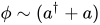
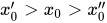
As the integral is in the time domain, one can Fourier transform it, together with the creation/annihilation operators, such that the amplitude eventually becomes

${\left\langle 0,x'_{0}|0,x''_{0}\right\rangle }_{J}=\exp {\left({\frac {i}{2\pi }}\int df~J(f){\frac {1}{f-E}}J(-f)\right)}.$

It is easy to notice that there is a singularity at $f=E$ . Then, we can exploit the $i\varepsilon$ -prescription and shift the pole $f-E+i\varepsilon$ such that for $x_{0}>x_{0}'$ the Green's function is revealed

${\begin{aligned}&{\left\langle 0|0\right\rangle }_{J}=\exp {\left({\frac {i}{2}}\int dx_{0}\,dx'_{0}\,J(x_{0})\Delta (x_{0}-x'_{0})J(x'_{0})\right)}\\[1ex]&\Delta (x_{0}-x'_{0})=\int {\frac {df}{2\pi }}{\frac {e^{-if\left(x_{0}-x'_{0}\right)}}{f-E+i\varepsilon }}\end{aligned}}$

The last result is the Schwinger's source theory for interacting scalar fields and can be generalized to any spacetime regions. The discussed examples below follow the metric $\eta _{\mu \nu }={\text{diag}}(1,-1,-1,-1)$ .

02Source theory for scalar fields

Causal perturbation theory explains how sources weakly act. For a weak source emitting spin-0 particles $J_{e}$ by acting on the vacuum state with a probability amplitude $\langle 0|0\rangle _{J_{e}}\sim 1$ , a single particle with momentum $p$ and amplitude $\langle p|0\rangle _{J_{e}}$ is created within certain spacetime region $x'$ . Then, another weak source $J_{a}$ absorbs that single particle within another spacetime region $x$ such that the amplitude becomes $\langle 0|p\rangle _{J_{a}}$ . Thus, the full vacuum amplitude is given by

${\left\langle 0|0\right\rangle }_{J_{e}+J_{a}}\sim 1+{\frac {i}{2}}\int dx\,dx'\,J_{a}(x)\Delta (x-x')J_{e}(x')$

where $\Delta (x-x')$ is the propagator (correlator) of the sources. The second term of the last amplitude defines the partition function of free scalar field theory. And for some interaction theory, the Lagrangian of a scalar field $\phi$ coupled to a current $J$ is given by

${\mathcal {L}}={\tfrac {1}{2}}\partial _{\mu }\phi \partial ^{\mu }\phi -{\tfrac {1}{2}}m^{2}\phi ^{2}+J\phi .$

If one adds $-i\varepsilon$ to the mass term then Fourier transforms both $J$ and $\phi$ to the momentum space, the vacuum amplitude becomes

$\langle 0|0\rangle =\exp {\left({\frac {i}{2}}\int {\frac {d^{4}p}{{\left(2\pi \right)}^{4}}}\left[{\tilde {\phi }}(p)\left(p_{\mu }p^{\mu }-m^{2}+i\varepsilon \right){\tilde {\phi }}(-p)+J(p){\frac {1}{p_{\mu }p^{\mu }-m^{2}+i\varepsilon }}J(-p)\right]\right)},$

where ${\tilde {\phi }}(p)=\phi (p)+{\frac {J(p)}{p_{\mu }p^{\mu }-m^{2}+i\varepsilon }}.$ It is easy to notice that the ${\tilde {\phi }}(p)\left(p_{\mu }p^{\mu }-m^{2}+i\varepsilon \right){\tilde {\phi }}(-p)$ term in the amplitude above can be Fourier transformed into ${\tilde {\phi }}(x)\left(\Box +m^{2}\right){\tilde {\phi }}(x)={\tilde {\phi }}(x)\,J(x)$ , i.e., the equation of motion $\left(\Box +m^{2}\right){\tilde {\phi }}=J$ . As the variation of the free action, that of the term ${\textstyle {\frac {1}{2}}\partial _{\mu }\phi \partial ^{\mu }\phi -{\frac {1}{2}}m^{2}\phi ^{2}$ , yields the equation of motion, one can redefine the Green's function as the inverse of the operator ${\textstyle G(x_{1},x_{2})\equiv {\left(\Box +m^{2}\right)}^{-1}$ such that $\left(\Box _{x_{1}}+m^{2}\right)G(x_{1},x_{2})=\delta (x_{1}-x_{2})$ if and only if ${\textstyle \left(p_{\mu }p^{\mu }-m^{2}\right)G(p)=1$ , which is a direct application of the general role of functional derivative ${\frac {\delta J(x_{2})}{\delta J(x_{1})}}=\delta (x_{1}-x_{2})$ . Thus, the generating functional is obtained from the partition function as follows. The last result allows us to read the partition function as ${\textstyle Z[J]=Z[0]\exp \left({\tfrac {i}{2}}\left\langle J(y)\Delta (y-y')J(y')\right\rangle \right)$ , where $Z[0]=\int {\mathcal {D}}{\tilde {\phi }}\,\exp \left(-i\int dt\left[{\tfrac {1}{2}}\partial _{\mu }{\tilde {\phi }}\partial ^{\mu }{\tilde {\phi }}-{\tfrac {1}{2}}\left(m^{2}-i\varepsilon \right){\tilde {\phi }}^{2}\right]\right),$ and $\langle J(y)\Delta (y-y')J(y')\rangle$ is the vacuum amplitude derived by the source $\langle 0|0\rangle _{J}$ . Consequently, the propagator is defined by varying the partition function as follows.

${\begin{aligned}{\left.{\frac {-1}{Z[0]}}{\frac {\delta ^{2}Z[J]}{\delta J(x)\delta J(x')}}\right\vert }_{J=0}&={\frac {-1}{2Z[0]}}{\frac {\delta }{\delta J(x)}}{\left[Z[J]\left(\int d^{4}y'\,\Delta (x'-y')J(y')+\int d^{4}y\,J(y)\Delta (y-x')\right)\right]}_{J=0}\\[1.5ex]&={\left.{\frac {Z[J]}{Z[0]}}\Delta (x-x')\right\vert }_{J=0}\\[1.5ex]&=\Delta (x-x').\end{aligned}}$

This motivates discussing the mean field approximation below.

03Effective action, mean field approximation, and vertex functions

Based on Schwinger's source theory, Steven Weinberg established the foundations of the effective field theory, which is widely appreciated among physicists. Despite the "shoes incident", Weinberg gave the credit to Schwinger for catalyzing this theoretical framework.

All Green's functions may be formally found via Taylor expansion of the partition sum considered as a function of the source fields. This method is commonly used in the path integral formulation of quantum field theory. The general method by which such source fields are utilized to obtain propagators in both quantum, statistical-mechanics and other systems is outlined as follows. Upon redefining the partition function in terms of Wick-rotated amplitude $W[J]=-i\ln(\langle 0|0\rangle _{J})$ , the partition function becomes $Z[J]=e^{iW[J]}$ . One can introduce $F[J]=iW[J]$ , which behaves as Helmholtz free energy in thermal field theories, to absorb the complex number, and hence $\ln Z[J]=F[J]$ . The function $F[J]$ is also called reduced quantum action. And with help of Legendre transform, we can invent a "new" effective energy functional, or effective action, as

$\Gamma [{\bar {\phi }}]=W[J]-\int d^{4}x\,J(x){\bar {\phi }}(x),$ with the transforms ${\begin{aligned}&{\frac {\delta W}{\delta J}}={\bar {\phi }}~,&&{\frac {\delta W}{\delta J}}{\Bigg |}_{J=0}=\langle \phi \rangle ~,\\[1.2ex]&{\frac {\delta \Gamma [{\bar {\phi }}]}{\delta {\bar {\phi }}}}{\Bigg |}_{J}=-J~,&&{\frac {\delta \Gamma [{\bar {\phi }}]}{\delta {\bar {\phi }}}}{\Bigg |}_{{\bar {\phi }}=\langle \phi \rangle }=0.\end{aligned}}$

The integration in the definition of the effective action is allowed to be replaced with sum over $\phi$ , i.e., $\Gamma [{\bar {\phi }}]=W[J]-J_{a}(x){\bar {\phi }}^{a}(x)$ . The last equation resembles the thermodynamical relation $F=E-TS$ between Helmholtz free energy and entropy. It is now clear that thermal and statistical field theories stem fundamentally from functional integrations and functional derivatives. Back to the Legendre transforms,

The $\langle \phi \rangle$ is called mean field obviously because $\langle \phi \rangle ={\frac {\int {\mathcal {D}}\phi ~e^{-i[\int dt~{\mathcal {L}}(t;\phi ,{\dot {\phi }})+\int dx^{4}J(x,t)\phi (x,t)]}~\phi ~}{Z[J]/{\mathcal {N}}}}$ , while ${\bar {\phi }}$ is a background classical field. A field $\phi$ is decomposed into a classical part ${\bar {\phi }}$ and fluctuation part $\eta$ , i.e., $\phi ={\bar {\phi }}+\eta$ , so the vacuum amplitude can be reintroduced as

$e^{i\Gamma [{\bar {\phi }}]}={\mathcal {N}}\int \exp \left[i\left(S[\phi ]-{\frac {\delta \Gamma [{\bar {\phi }}]}{\delta {\bar {\phi }}}}\eta \right)\right]d\phi ,$

and any function ${\mathcal {F}}[\phi ]$ is defined as

$\langle {\mathcal {F}}[\phi ]\rangle =e^{-i\Gamma [{\bar {\phi }}]}~{\mathcal {N}}\int {\mathcal {F}}[\phi ]\exp \left[i\left(S[\phi ]-{\frac {\delta \Gamma [{\bar {\phi }}]}{\delta {\bar {\phi }}}}\eta \right)\right]d\phi ,$

where $S[\phi ]$ is the action of the free Lagrangian. The last two integrals are the pillars of any effective field theory. This construction is indispensable in studying scattering (LSZ reduction formula), spontaneous symmetry breaking, Ward identities, nonlinear sigma models, and low-energy effective theories. Additionally, this theoretical framework initiates line of thoughts, publicized mainly be Bryce DeWitt who was a PhD student of Schwinger, on developing a canonical quantized effective theory for quantum gravity.

Back to Green functions of the actions. Since $\Gamma [{\bar {\phi }}]$ is the Legendre transform of $F[J]$ , and $F[J]$ defines N-points connected correlator $G_{F[J]}^{N,~c}={\frac {\delta F[J]}{\delta J(x_{1})\cdots \delta J(x_{N})}}{\Big |}_{J=0}$ , then the corresponding correlator obtained from $F[J]$ , known as vertex function, is given by $G_{\Gamma [J]}^{N,~c}=\left.{\frac {\delta \Gamma [{\bar {\phi }}]}{\delta {\bar {\phi }}(x_{1})\cdots \delta {\bar {\phi }}(x_{N})}}\right|_{{\bar {\phi }}=\langle \phi \rangle }$ . Consequently, in the one particle irreducible graphs (usually acronymized as 1PI), the connected 2-point $F$ -correlator is defined as the inverse of the 2-point $\Gamma$ -correlator, i.e., the usual reduced correlation is $G_{F[J]}^{(2)}={\frac {\delta {\bar {\phi }}(x_{1})}{\delta J(x_{2})}}{\Big |}_{J=0}={\frac {1}{p_{\mu }p^{\mu }-m^{2}}}$ , and the effective correlation is $G_{\Gamma [\phi ]}^{(2)}={\frac {\delta J(x_{1})}{\delta {\bar {\phi }}(x_{2})}}{\Big |}_{{\bar {\phi }}=\langle \phi \rangle }=p_{\mu }p^{\mu }-m^{2}$ . For $J_{i}=J(x_{i})$ , the most general relations between the N-points connected $F[J]$ and $Z[J]$ are obtained from Faà di Bruno's formula

${\begin{aligned}{\frac {\delta ^{N}F}{\delta J_{1}\cdots \delta J_{N}}}=&{\frac {1}{Z[J]}}{\frac {\delta ^{N}Z[J]}{\delta J_{1}\cdots \delta J_{N}}}-{\Big \{}{\frac {1}{Z^{2}[J]}}{\frac {\delta Z[J]}{\delta J_{1}}}{\frac {\delta ^{N-1}Z[J]}{\delta J_{2}\cdots \delta J_{N}}}+{\text{perm}}{\Big \}}+{\big \{}{\frac {1}{Z^{3}[J]}}{\frac {\delta Z[J]}{\delta J_{1}}}{\frac {\delta Z[J]}{\delta J_{2}}}{\frac {\delta ^{N-2}Z[J]}{\delta J_{3}\cdots \delta J_{N}}}+{\text{perm}}{\Big \}}+\cdots \\&-{\Big \{}{\frac {1}{Z^{2}[J]}}{\frac {\delta ^{2}Z[J]}{\delta J_{1}\delta J_{2}}}{\frac {\delta ^{N-2}Z[J]}{\delta J_{3}\cdots \delta J_{N}}}+{\text{perm}}{\Big \}}+{\Big \{}{\frac {1}{Z^{3}[J]}}{\frac {\delta ^{3}Z[J]}{\delta J_{1}\delta J_{2}\delta J_{3}}}{\frac {\delta ^{N-3}Z[J]}{\delta J_{4}\cdots \delta J_{N}}}+{\text{perm}}{\Big \}}-\cdots \end{aligned}}$

and

${\begin{aligned}{\frac {1}{Z[J]}}{\frac {\delta ^{N}Z[J]}{\delta J_{1}\cdots \delta J_{N}}}=&{\frac {\delta ^{N}F[J]}{\delta J_{1}\cdots \delta J_{N}}}+{\Big \{}{\frac {\delta F[J]}{\delta J_{1}}}{\frac {\delta ^{N-1}F[J]}{\delta J_{2}\cdots \delta J_{N}}}+{\text{perm}}{\Big \}}+{\Big \{}{\frac {\delta F[J]}{\delta J_{1}}}{\frac {\delta F[J]}{\delta J_{2}}}{\frac {\delta ^{N-2}F[J]}{\delta J_{3}\cdots \delta J_{N}}}+{\text{perm}}{\Big \}}+\cdots \\&+{\Big \{}{\frac {\delta ^{2}F[J]}{\delta J_{1}\delta J_{2}}}{\frac {\delta ^{N-2}F[J]}{\delta J_{3}\cdots \delta J_{N}}}+{\text{perm}}{\Big \}}+{\Big \{}{\frac {\delta ^{3}F[J]}{\delta J_{1}\delta J_{2}\delta J_{3}}}{\frac {\delta ^{N-3}F[J]}{\delta J_{4}\cdots \delta J_{N}}}+{\text{perm}}{\Big \}}+\cdots \end{aligned}}$

04Source theory for fields

Vector fields

For a weak source producing a massive spin-1 particle with a general current $J=J_{e}+J_{a}$ acting on different causal spacetime points $x_{0}>x_{0}'$ , the vacuum amplitude is

$\langle 0|0\rangle _{J}=\exp {\left({\frac {i}{2}}\int dx~dx'\left[J_{\mu }(x)\Delta (x-x')J^{\mu }(x')+{\frac {1}{m^{2}}}\partial _{\mu }J^{\mu }(x)\Delta (x-x')\partial '_{\nu }J^{\nu }(x')\right]\right)}$

In momentum space, the spin-1 particle with rest mass $m$ has a definite momentum $p_{\mu }=(m,0,0,0)$ in its rest frame, i.e. $p_{\mu }p^{\mu }=m^{2}$ . Then, the amplitude gives

${\begin{alignedat}{2}(J_{\mu }(p))^{T}~J^{\mu }(p)-{\frac {1}{m^{2}}}(p_{\mu }J^{\mu }(p))^{T}~p_{\nu }J^{\nu }(p)&=(J_{\mu }(p))^{T}~J^{\mu }(p)-(J^{\mu }(p))^{T}~{\frac {p_{\mu }p_{\nu }}{p_{\sigma }p^{\sigma }}}{\bigg |}_{\text{on-shell}}~J^{\nu }(p)\\&=(J^{\mu }(p))^{T}~\left[\eta _{\mu \nu }-{\frac {p_{\mu }p_{\nu }}{m^{2}}}\right]~J^{\nu }(p)\end{alignedat}}$

where $\eta _{\mu \nu }={\text{diag}}(1,-1,-1,-1)$ and $(J_{\mu }(p))^{T}$ is the transpose of $J_{\mu }(p)$ . The last result matches with the used propagator in the vacuum amplitude in the configuration space, that is,

$\left\langle 0\right|TA_{\mu }(x)A_{\nu }(x')\left|0\right\rangle =-i\int {\frac {d^{4}p}{{\left(2\pi \right)}^{4}}}{\frac {1}{p_{\alpha }p^{\alpha }+i\varepsilon }}\left[\eta _{\mu \nu }-\left(1-\xi \right){\frac {p_{\mu }p_{\nu }}{p_{\sigma }p^{\sigma }-\xi m^{2}}}\right]e^{ip^{\mu }\left(x_{\mu }-x'_{\mu }\right)}.$

When $\xi =1$ , the chosen Feynman-'t Hooft gauge-fixing makes the spin-1 massless. And when $\xi =0$ , the chosen Landau gauge-fixing makes the spin-1 massive. The massless case is obvious as studied in quantum electrodynamics. The massive case is more interesting as the current is not demanded to conserved. However, the current can be improved in a way similar to how the Belinfante-Rosenfeld tensor is improved so it ends up being conserved. And to get the equation of motion for the massive vector, one can define

$W[J]=-i\ln(\langle 0|0\rangle _{J})={\frac {1}{2}}\int dx~dx'\left[J_{\mu }(x)\Delta (x-x')J^{\mu }(x')+{\frac {1}{m^{2}}}\partial _{\mu }J^{\mu }(x)\Delta (x-x')\partial '_{\nu }J^{\nu }(x')\right].$

One can apply integration by part on the second term then single out ${\textstyle \int dxJ_{\mu }(x)$ to get a definition of the massive spin-1 field

$A_{\mu }(x)\equiv \int dx'\Delta (x-x')J^{\mu }(x')-{\frac {1}{m^{2}}}\partial _{\mu }\left[\int dx'\Delta (x-x')\partial '_{\nu }J^{\nu }(x')\right].$

Additionally, the equation above says that ${\textstyle \partial _{\mu }A^{\mu }={\tfrac {1}{m^{2}}}\partial _{\mu }J^{\mu }$ . Thus, the equation of motion can be written in any of the following forms

${\begin{aligned}&\left(\Box +m^{2}\right)A_{\mu }=J_{\mu }+{\tfrac {1}{m^{2}}}\partial _{\nu }\partial _{\mu }J^{\nu },\\[1ex]&\left(\Box +m^{2}\right)A_{\mu }+\partial _{\nu }\partial _{\mu }A^{\nu }=J_{\mu }.\end{aligned}}$

Massive totally symmetric spin-2 fields

For a weak source in a flat Minkowski background, producing then absorbing a massive spin-2 particle with a general redefined energy-momentum tensor, acting as a current, ${\textstyle {\bar {T}}^{\mu \nu }=T^{\mu \nu }-{\tfrac {1}{3}}\eta _{\mu \alpha }{\bar {\eta }}_{\nu \beta }T^{\alpha \beta }$ , where ${\textstyle {\bar {\eta }}_{\mu \nu }(p)=\eta _{\mu \nu }-{\tfrac {1}{m^{2}}}p_{\mu }p_{\nu }$ is the vacuum polarization tensor, the vacuum amplitude in a compact form is

${\begin{aligned}\langle 0|0\rangle _{\bar {T}}=\exp {\Biggl (}-{\frac {i}{2}}\int {\biggl [}&{\bar {T}}_{\mu \nu }(x)\Delta (x-x'){\bar {T}}^{\mu \nu }(x')\\&+{\frac {2}{m^{2}}}\eta _{\lambda \nu }\partial _{\mu }{\bar {T}}^{\mu \nu }(x)\Delta (x-x')\partial '_{\kappa }{\bar {T}}^{\kappa \lambda }(x')\\&+{\frac {1}{m^{4}}}\partial _{\mu }\partial _{\nu }{\bar {T}}^{\mu \nu }(x)\Delta (x-x')\partial '_{\kappa }\partial '_{\lambda }{\bar {T}}^{\kappa \lambda }(x'){\biggr ]}dx\,dx'{\Biggr )},\end{aligned}}$

${\begin{aligned}\langle 0|0\rangle _{T}=\exp {\Biggl (}-{\frac {i}{2}}\int {\biggl [}&T_{\mu \nu }(x)\Delta (x-x')T^{\mu \nu }(x')\\&+{\frac {2}{m^{2}}}\eta _{\lambda \nu }\partial _{\mu }T^{\mu \nu }(x)\Delta (x-x')\partial '_{\kappa }T^{\kappa \lambda }(x')\\&+{\frac {1}{m^{4}}}\partial _{\mu }\partial _{\mu }T^{\mu \nu }(x)\Delta (x-x')\partial '_{\kappa }\partial '_{\lambda }T^{\kappa \lambda }(x')\\&-{\frac {1}{3}}\left(\eta _{\mu \nu }T^{\mu \nu }(x)-{\frac {1}{m^{2}}}\partial _{\mu }\partial _{\nu }T^{\mu \nu }(x)\right)\Delta (x-x')\left(\eta _{\kappa \lambda }T^{\kappa \lambda }(x')-{\frac {1}{m^{2}}}\partial '_{\kappa }\partial '_{\lambda }T^{\kappa \lambda }(x')\right){\biggr ]}dx~dx'{\Biggr )}.\end{aligned}}$

This amplitude in momentum space gives (transpose is imbedded)

${\begin{aligned}{\bar {T}}_{\mu \nu }(p)\eta ^{\mu \kappa }\eta ^{\nu \lambda }{\bar {T}}_{\kappa \lambda }(p)&-{\frac {1}{m^{2}}}{\bar {T}}_{\mu \nu }(p)\eta ^{\mu \kappa }p^{\nu }p^{\lambda }{\bar {T}}_{\kappa \lambda }(p)\\&-{\frac {1}{m^{2}}}{\bar {T}}_{\mu \nu }(p)\eta ^{\nu \lambda }p^{\mu }p^{\kappa }{\bar {T}}_{\kappa \lambda }(p)+{\frac {1}{m^{4}}}{\bar {T}}_{\mu \nu }(p)p^{\mu }p^{\nu }p^{\kappa }p^{\lambda }{\bar {T}}_{\kappa \lambda }(p)=\end{aligned}}$

${\begin{aligned}\eta ^{\mu \kappa }{\biggl (}{\bar {T}}_{\mu \nu }(p)\eta ^{\nu \lambda }{\bar {T}}_{\kappa \lambda }(p)&-{\frac {1}{m^{2}}}{\bar {T}}_{\mu \nu }(p)p^{\nu }p^{\lambda }{\bar {T}}_{\kappa \lambda }(p){\biggr )}\\&-{\frac {1}{m^{2}}}p^{\mu }p^{\kappa }\left({\bar {T}}_{\mu \nu }(p)\eta ^{\nu \lambda }{\bar {T}}_{\kappa \lambda }(p)-{\frac {1}{m^{2}}}{\bar {T}}_{\mu \nu }(p)p^{\nu }p^{\lambda }{\bar {T}}_{\kappa \lambda }(p)\right)\\=\left(\eta ^{\mu \kappa }-{\frac {1}{m^{2}}}p^{\mu }p^{\kappa }\right)&\left({\bar {T}}_{\mu \nu }(p)\eta ^{\nu \lambda }{\bar {T}}_{\kappa \lambda }(p)-{\frac {1}{m^{2}}}{\bar {T}}_{\mu \nu }(p)p^{\nu }p^{\lambda }{\bar {T}}_{\kappa \lambda }(p)\right)\\=&{\bar {T}}_{\mu \nu }(p)\left(\eta ^{\mu \kappa }-{\frac {1}{m^{2}}}p^{\mu }p^{\kappa }\right)\left(\eta ^{\nu \lambda }-{\frac {1}{m^{2}}}p^{\nu }p^{\lambda }\right){\bar {T}}_{\kappa \lambda }(p).\end{aligned}}$

And with help of symmetric properties of the source, the last result can be written as $T^{\mu \nu }(p)\Pi _{\mu \nu \kappa \lambda }(p)T^{\kappa \lambda }(p)$ , where the projection operator, or the Fourier transform of Jacobi field operator obtained by applying Peierls braket on Schwinger's variational principle, is ${\textstyle \Pi _{\mu \nu \kappa \lambda }(p)={\tfrac {1}{2}}\left({\bar {\eta }}_{\mu \kappa }(p){\bar {\eta }}_{\nu \lambda }(p)+{\bar {\eta }}_{\mu \lambda }(p){\bar {\eta }}_{\nu \kappa }(p)-{\tfrac {2}{3}}{\bar {\eta }}_{\mu \nu }(p){\bar {\eta }}_{\kappa \lambda }(p)\right)$ .

In N-dimensional flat spacetime, 2/3 is replaced by 2/(N−1). And for massless spin-2 fields, the projection operator is defined as $\Pi _{\mu \nu \kappa \lambda }^{m=0}={\tfrac {1}{2}}\left(\eta _{\mu \kappa }\eta _{\nu \lambda }+\eta _{\mu \lambda }\eta _{\nu \kappa }-{\tfrac {1}{2}}\eta _{\mu \nu }\eta _{\kappa \lambda }\right)$ .

Together with help of Ward-Takahashi identity, the projector operator is crucial to check the symmetric properties of the field, the conservation law of the current, and the allowed physical degrees of freedom.

It is worth noting that the vacuum polarization tensor ${\bar {\eta }}_{\nu \beta }$ and the improved energy momentum tensor ${\bar {T}}^{\mu \nu }$ appear in the early versions of massive gravity theories. Interestingly, massive gravity theories have not been widely appreciated until recently due to apparent inconsistencies obtained in the early 1970s studies of the exchange of a single spin-2 field between two sources. But in 2010 the dRGT approach of exploiting Stueckelberg field redefinition led to consistent covariantized massive theory free of all ghosts and discontinuities obtained earlier.

If one looks at $\langle 0|0\rangle _{T}$ and follows the same procedure used to define massive spin-1 fields, then it is easy to define massive spin-2 fields as

${\begin{aligned}h_{\mu \nu }(x)=&\int \Delta (x-x')T_{\mu \nu }(x')dx'\\&-{\frac {1}{m^{2}}}\partial _{\mu }\int \Delta (x-x')\partial '^{\kappa }T_{\kappa \nu }(x')dx'\\&-{\frac {1}{m^{2}}}\partial _{\nu }\int \Delta (x-x')\partial '^{\kappa }T_{\kappa \mu }(x')dx'\\&+{\frac {1}{m^{4}}}\partial _{\mu }\partial _{\nu }\int \Delta (x-x')\partial '_{\kappa }\partial '_{\lambda }T^{\kappa \lambda }(x')dx'\\&-{\frac {1}{3}}\left(\eta _{\mu \nu }-{\frac {1}{m^{2}}}\partial _{\mu }\partial _{\nu }\right)\int \Delta (x-x')\left[\eta _{\kappa \lambda }T^{\kappa \lambda }(x')-{\frac {1}{m^{2}}}\partial '_{\kappa }\partial '_{\lambda }T^{\kappa \lambda }(x')\right]dx'.\end{aligned}}$

The corresponding divergence condition is read 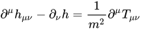$\partial ^{\mu }h_{\mu \nu }-\partial _{\nu }h={\frac {1}{m^{2}}}\partial ^{\mu }T_{\mu \nu }$ , where the current $\partial ^{\mu }T_{\mu \nu }$ is not necessarily conserved (it is not a gauge condition as that of the massless case). But the energy-momentum tensor can be improved as ${\textstyle {\mathfrak {T}}_{\mu \nu }=T_{\mu \nu }-{\frac {1}{4}}\eta _{\mu \nu }{\mathfrak {T}}$ such that $\partial ^{\mu }{\mathfrak {T}}_{\mu \nu }=0$ according to Belinfante-Rosenfeld construction. Thus, the equation of motion

${\begin{aligned}\left(\square +m^{2}\right)h_{\mu \nu }=T_{\mu \nu }&+{\dfrac {1}{m^{2}}}\left(\partial _{\mu }\partial ^{\rho }T_{\rho \nu }+\partial _{\nu }\partial ^{\rho }T_{\rho \mu }-{\frac {1}{2}}\eta _{\mu \nu }\partial ^{\rho }\partial ^{\sigma }T_{\rho \sigma }\right)\\&+{\frac {2}{3m^{4}}}\left(\partial _{\mu }\partial _{\nu }-{\frac {1}{4}}\eta _{\mu \nu }\square \right)\partial ^{\rho }\partial ^{\sigma }T_{\rho \sigma }\end{aligned}}$

becomes

$\left(\square +m^{2}\right)h_{\mu \nu }={\mathfrak {T}}_{\mu \nu }-{\frac {1}{4}}~\eta _{\mu \nu }{\mathfrak {T}}-{\dfrac {1}{6m^{4}}}\left(\partial _{\mu }\partial _{\nu }-{\frac {1}{4}}~\eta _{\mu \nu }\square \right)\left(\square +3m^{2}\right){\mathfrak {T}}.$

One can use the divergence condition to decouple the non-physical fields $\partial ^{\mu }h_{\mu \nu }$ and $h$ , so the equation of motion is simplified as

$\left(\square +m^{2}\right)h_{\mu \nu }={\mathfrak {T}}_{\mu \nu }-{\frac {1}{3}}~\eta _{\mu \nu }{\mathfrak {T}}-{\frac {1}{3m^{2}}}~\partial _{\mu }\partial _{\nu }{\mathfrak {T}}.$

Massive totally symmetric arbitrary integer spin fields

One can generalize $T^{\mu \nu }(p)$ source to become $S^{\mu _{1}\cdots \mu _{\ell }}(p)$ higher-spin source such that $T^{\mu \nu }(p)\Pi _{\mu \nu \kappa \lambda }(p)T^{\kappa \lambda }(p)$ becomes $S^{\mu _{1}\cdots \mu _{\ell }}(p)\Pi _{\mu _{1}\cdots \mu _{\ell }\nu _{1}\cdots \nu _{\ell }}(p)S^{\nu _{1}\cdots \nu _{\ell }}(p)$ . The generalized projection operator also helps generalizing the electromagnetic polarization vector $e_{m}^{\mu }(p)$ of the quantized electromagnetic vector potential as follows. For spacetime points $x$ and $x'$ , the addition theorem of spherical harmonics states that

$x^{\mu _{1}}\cdots x^{\mu _{\ell }}\Pi _{\mu _{1}\cdots \mu _{\ell }\nu _{1}\cdots \nu _{\ell }}(p)x'^{\nu _{1}}\cdots x'^{\nu _{\ell }}={\frac {2^{\ell }(\ell !)^{2}}{(2\ell )!}}{\frac {4\pi }{2\ell +1}}\sum \limits _{m=-\ell }^{\ell }Y_{\ell ,m}(x)Y_{\ell ,m}^{*}(x').$

Also, the representation theory of the space of complex-valued homogeneous polynomials of degree $\ell$ on a unit (N-1)-sphere defines the polarization tensor as $e_{(m)}(x_{1},\dots ,x_{n})=\sum _{i_{1}\dots i_{\ell }}e_{(m)i_{1}\dots i_{\ell }}x_{i_{1}}\cdots x_{i_{\ell }},~\forall x_{i}\in S^{N-1}.$ Then, the generalized polarization vector is $e^{\mu _{1}\cdots \mu _{\ell }}(p)~x_{\mu _{1}}\cdots x_{\mu _{\ell }}={\sqrt {{\frac {2^{\ell }(\ell !)^{2}}{(2\ell )!}}{\frac {4\pi }{2\ell +1}}}}~~Y_{\ell ,m}(x).$

And the projection operator can be defined as $\Pi ^{\mu _{1}\cdots \mu _{\ell }\nu _{1}\cdots \nu _{\ell }}(p)=\sum \limits _{m=-\ell }^{\ell }[e_{m}^{\mu _{1}\cdots \mu _{\ell }}(p)]~[e_{m}^{\nu _{1}\cdots \nu _{\ell }}(p)]^{*}.$

The symmetric properties of the projection operator make it easier to deal with the vacuum amplitude in the momentum space. Therefore, rather that we express it in terms of the correlator $\Delta (x-x')$ in configuration space, we write

$\langle 0|0\rangle _{S}=\exp {\left[{\frac {i}{2}}\int {\frac {dp^{4}}{(2\pi )^{4}}}S^{\mu _{1}\cdots \mu _{\ell }}(-p){\frac {\Pi _{\mu _{1}\cdots \mu _{\ell }\nu _{1}\cdots \nu _{\ell }}(p)}{p_{\sigma }p^{\sigma }-m^{2}+i\varepsilon }}S^{\nu _{1}\cdots \nu _{\ell }}(p)\right]}.$

Mixed symmetric arbitrary spin fields

Also, it is theoretically consistent to generalize the source theory to describe hypothetical gauge fields with antisymmetric and mixed symmetric properties in arbitrary dimensions and arbitrary spins. But one should take care of the unphysical degrees of freedom in the theory. For example, in N-dimensions and for a mixed symmetric massless version of Curtright field $T_{[\mu \nu ]\lambda }$ and a source $S_{[\mu \nu ]\lambda }=\partial _{\alpha }\partial ^{\alpha }T_{[\mu \nu ]\lambda }$ , the vacuum amplitude is $\langle 0|0\rangle _{S}=\exp {\left(-{\frac {1}{2}}\int dx~dx'\left[S_{[\mu \nu ]\lambda }(x)\Delta (x-x')S_{[\mu \nu ]\lambda }(x')+{\frac {2}{3-N}}S_{[\mu \alpha ]\alpha }(x)\Delta (x-x')S_{[\mu \beta ]\beta }(x')\right]\right)}$ which for a theory in N=4 makes the source eventually reveal that it is a theory of a non physical field. However, the massive version survives in N≥5.

Arbitrary half-integer spin fields

For spin-1⁄2 fermion propagator $S(x-x')=(p\!\!\!/+m)\Delta (x-x')$ and current $J=J_{e}+J_{a}$ as defined above, the vacuum amplitude is

${\begin{aligned}\langle 0|0\rangle _{J}&=\exp {\left[{\frac {i}{2}}\int dxdx'~J(x)~\left(\gamma ^{0}S(x-x')\right)~J(x')\right]}\\&=\langle 0|0\rangle _{J_{e}}\exp {\left[i\int dxdx'~J_{e}(x)~\left(\gamma ^{0}S(x-x')~\right)~J_{a}(x')\right]}\langle 0|0\rangle _{J_{a}}.\end{aligned}}$

In momentum space the reduced amplitude is given by

$W_{\frac {1}{2}}=-{\frac {1}{3}}\int {\frac {d^{4}p}{(2\pi )^{4}}}~J(-p)\left[\gamma ^{0}{\frac {p\!\!\!/+m}{p^{2}-m^{2}}}\right]~J(p).$

For spin-3⁄2 Rarita-Schwinger fermions, ${\textstyle \Pi _{\mu \nu }={\bar {\eta }}_{\mu \nu }-{\tfrac {1}{3}}\gamma ^{\alpha }{\bar {\eta }}_{\alpha \mu }\gamma ^{\beta }{\bar {\eta }}_{\beta \nu }.$ Then, one can use $\gamma _{\mu }=\eta _{\mu \nu }\gamma ^{\nu }$ and the on-shell $p\!\!\!/=-m$ to get

${\begin{aligned}W_{\frac {3}{2}}&=-{\frac {2}{5}}\int {\frac {d^{4}p}{{\left(2\pi \right)}^{4}}}\,J^{\mu }(-p)\left[\gamma ^{0}{\frac {(p\!\!\!/+m)\left({\bar {\eta }}_{\mu \nu }|_{\text{on-shell}}-{\frac {1}{3}}\gamma ^{\alpha }{\bar {\eta }}_{\alpha \mu }|_{\text{on-shell}}\gamma ^{\beta }{\bar {\eta }}_{\beta \nu }|_{\text{on-shell}}\right)}{p^{2}-m^{2}}}\right]~J^{\nu }(p)\\&=-{\frac {2}{5}}\int {\frac {d^{4}p}{{\left(2\pi \right)}^{4}}}\,J^{\mu }(-p)\left[\gamma ^{0}{\frac {\left(\eta _{\mu \nu }-{\frac {p_{\mu }p_{\nu }}{m^{2}}}\right)(p\!\!\!/+m)-{\frac {1}{3}}\left(\gamma _{\mu }+{\frac {1}{m}}p_{\mu }\right)\left(p\!\!\!/+m\right)\left(\gamma _{\nu }+{\frac {1}{m}}p_{\nu }\right)}{p^{2}-m^{2}}}\right]~J^{\nu }(p).\end{aligned}}$

One can replace the reduced metric ${\bar {\eta }}_{\mu \nu }$ with the usual one $\eta _{\mu \nu }$ if the source $J_{\mu }$ is replaced with ${\bar {J}}_{\mu }(p)={\frac {2}{5}}\gamma ^{\alpha }\Pi _{\mu \alpha \nu \beta }\gamma ^{\beta }J^{\nu }(p).$

For spin- $(j+{\tfrac {1}{2}})$ , the above results can be generalized to

$W_{j+{\frac {1}{2}}}=-{\frac {j+1}{2j+3}}\int {\frac {d^{4}p}{{\left(2\pi \right)}^{4}}}\,J^{\mu _{1}\cdots \mu _{j}}(-p)~\left[\gamma ^{0}{\frac {~\gamma ^{\alpha }~\Pi _{\mu _{1}\cdots \mu _{j}\alpha \nu _{1}\cdots \nu _{j}\beta }~\gamma ^{\beta }}{p^{2}-m^{2}}}\right]J^{\nu _{1}\cdots \nu _{j}}(p).$

The factor ${\frac {j+1}{2j+3}}$ is obtained from the properties of the projection operator, the tracelessness of the current, and the conservation of the current after being projected by the operator. These conditions can be derived from the Fierz-Pauli and the Fang-Fronsdal conditions on the fields themselves. The Lagrangian formulations of massive fields and their conditions were studied by Lambodar Singh and Carl Hagen. The non-relativistic version of the projection operators, developed by Charles Zemach who is another student of Schwinger, is used heavily in hadron spectroscopy. Zemach's method could be relativistically improved to render the covariant projection operators.

Watch videos about Source fieldExplainers and documentaries on YouTube (opens in a new tab)

Sources and credits

This article is adapted from the Wikipedia article “Source field”, written by its contributors and licensed under CC BY-SA 4.0. Fathomly has changed the layout, removed citation markers, navigation and maintenance notices, and adjusted punctuation. This adapted version is shared under the same license. For references, see the original article.

Fathomly is not affiliated with or endorsed by the Wikimedia Foundation. Spotted a problem? Tell us.