Encyclopedia

Set cover problem

Classical problem in combinatorics

Wikipedia contributorsAdapted for Fathomly · View authors

10 min read
Source updated August 11, 2026

The set cover problem is a classical question in combinatorics, computer science, operations research, and complexity theory.

Given a set of elements {1, 2, …, n} (henceforth referred to as the universe, specifying all possible elements under consideration) and a collection, referred to as S, of a given m subsets whose union equals the universe, the set cover problem is to identify a smallest sub-collection of S whose union equals the universe.

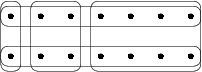
For example, consider the universe, U = {1, 2, 3, 4, 5} and the collection of sets S = { {1, 2, 3}, {2, 4}, {3, 4}, {4, 5} }. In this example, m is equal to 4, as there are four subsets that comprise this collection. The union of S is equal to U. However, we can cover all elements with only two sets: { {1, 2, 3}, {4, 5} }‍, but not with only one set. Therefore, the solution to the set cover problem for this U and S has size 2. This example is illustrated in the picture above.

More formally, given a universe ${\mathcal {U}}$ and a family ${\mathcal {S}}$ of subsets of ${\mathcal {U}}$ , a set cover is a subfamily ${\mathcal {C}}\subseteq {\mathcal {S}}$ of sets whose union is ${\mathcal {U}}$ .

In the set cover decision problem, the input is a pair $({\mathcal {U}},{\mathcal {S}})$ and an integer $k$ ; the question is whether there is a set cover of size $k$ or less.
In the set cover optimization problem, the input is a pair $({\mathcal {U}},{\mathcal {S}})$ , and the task is to find a set cover that uses the fewest sets.

The decision version of set covering is NP-complete. It is one of Karp's 21 NP-complete problems shown to be NP-complete in 1972. The optimization/search version of set cover is NP-hard. It is a problem "whose study has led to the development of fundamental techniques for the entire field" of approximation algorithms.

01Variants

In the weighted set cover problem, each set is assigned a positive weight (representing its cost), and the goal is to find a set cover with a smallest weight. The usual (unweighted) set cover corresponds to all sets having a weight of 1.

In the fractional set cover problem, it is allowed to select fractions of sets, rather than entire sets. A fractional set cover is an assignment of a fraction (a number in [0,1]) to each set in ${\mathcal {S}}$ , such that for each element x in the universe, the sum of fractions of sets that contain x is at least 1. The goal is to find a fractional set cover in which the sum of fractions is as small as possible. Note that a (usual) set cover is equivalent to a fractional set cover in which all fractions are either 0 or 1; therefore, the size of the smallest fractional cover is at most the size of the smallest cover, but may be smaller. For example, consider the universe U = {1, 2, 3} and the collection of sets S = { {1, 2}, {2, 3}, {3, 1} }. The smallest set cover has a size of 2, e.g. { {1, 2}, {2, 3} }. But there is a fractional set cover of size 1.5, in which a 0.5 fraction of each set is taken.

In the capacitated set cover problem, each set $s\in {\mathcal {S}}$ is associated with a capacity $c_{S}$ which denotes the number of elements it can supply coverage. The goal is to determine the optimal way to select sets such that each element receives the coverage it requires.

Tight example for the greedy algorithm with k=3

02Linear program formulation

The set cover problem can be formulated as the following integer linear program (ILP).

minimize	$\sum _{s\in {\mathcal {S}}}x_{s}$		(minimize the number of sets)
subject to	$\sum _{s\colon e\in s}x_{s}\geqslant 1$	for all $e\in {\mathcal {U}}$	(cover every element of the universe)
	$x_{s}\in \{0,1\}$	for all $s\in {\mathcal {S}}$ .	(every set is either in the set cover or not)

For a more compact representation of the covering constraint, one can define an incidence matrix $A$ , where each row corresponds to an element and each column corresponds to a set, and $A_{e,s}=1$ if element e is in set s, and $A_{e,s}=0$ otherwise. Then, the covering constraint can be written as $Ax\geqslant 1$ .

Weighted set cover is described by a program identical to the one given above, except that the objective function to minimize is $\sum _{s\in {\mathcal {S}}}w_{s}x_{s}$ , where $w_{s}$ is the weight of set $s\in {\mathcal {S}}$ .

Fractional set cover is described by a program identical to the one given above, except that $x_{s}$ can be non-integer, so the last constraint is replaced by $0\leq x_{s}\leq 1$ .

This linear program belongs to the more general class of LPs for covering problems, as all the coefficients in the objective function and both sides of the constraints are non-negative. The integrality gap of the ILP is at most $\scriptstyle \log n$ (where $\scriptstyle n$ is the size of the universe). It has been shown that its relaxation indeed gives a factor- $\scriptstyle \log n$ approximation algorithm for the minimum set cover problem. See setcover for a detailed explanation.

03Hitting set formulation

The set cover problem is equivalent to the hitting set problem. A subset $H$ of $U$ is called a hitting set when $H\cap S_{j}\neq \emptyset$ for all $1\leq j\leq m$ (i.e., $H$ intersects or "hits" all subsets in $S$ ). The hitting set problem is to find a minimum hitting set $H$ for a given $U$ and $S$ .

To show that the problems are equivalent, for a universe $U$ of size $n$ and collection of sets $S$ of size $m$ , construct $U'=\{1,2,\ldots ,m\}$ and $S'_{i}=\{j\mid i\in S_{j}\}$ . Then a set cover $C$ of $S$ is equivalent to a hitting set $H'$ of $U'$ where $S_{j}\in C\iff j\in H'$ , and vice versa.

This equivalence can also be visualized by representing the problem as a bipartite graph of $n+m$ vertices, with $n$ vertices on the left representing elements of $U$ , and $m$ vertices on the right representing elements of $S$ , and edges representing set membership (i.e., there is an edge between the $i$ -th vertex on the left and the $j$ -th vertex of the right iff. $i\in S_{j}$ ). Then a set cover is a subset $C$ of right vertices such that each left vertex is adjacent to at least one member of $C$ , while a hitting set is a subset $H$ of left vertices such that each right vertex is adjacent to at least one member of $H$ . These definitions are exactly the same except that left and right are swapped. But there is nothing special about the sides in the bipartite graph; we could have put the elements of $U$ on the right side, and the elements of $S$ on the left side, creating a graph that is a mirror image of the one described above. This shows that set covers in the original graph are equivalent to hitting sets in the mirrored graph, and vice versa.

In the field of computational geometry, a hitting set for a collection of geometrical objects is also called a stabbing set or piercing set.

04Greedy algorithm

There is a greedy algorithm for polynomial time approximation of set covering that chooses sets according to one rule: at each stage, choose the set that contains the largest number of uncovered elements. This method can be implemented in time linear in the sum of sizes of the input sets, using a bucket queue to prioritize the sets. It achieves an approximation ratio of $H(s)$ , where $s$ is the size of the set to be covered. In other words, it finds a covering that may be $H(n)$ times as large as the minimum one, where $H(n)$ is the $n$ -th harmonic number: $H(n)=\sum _{k=1}^{n}{\frac {1}{k}}\leq \ln {n}+1$

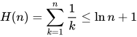
This greedy algorithm actually achieves an approximation ratio of $H(s^{\prime })$ where $s^{\prime }$ is the maximum cardinality set of $S$ . For $\delta -$ dense instances, however, there exists a $c\ln {m}$ -approximation algorithm for every $c>0$ .

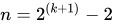
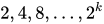
There is a standard example on which the greedy algorithm achieves an approximation ratio of $\log _{2}(n)/2$ . The universe consists of $n=2^{(k+1)}-2$ elements. The set system consists of $k$ pairwise disjoint sets $S_{1},\ldots ,S_{k}$ with sizes $2,4,8,\ldots ,2^{k}$ respectively, as well as two additional disjoint sets $T_{0},T_{1}$ , each of which contains half of the elements from each $S_{i}$ . On this input, the greedy algorithm takes the sets $S_{k},\ldots ,S_{1}$ , in that order, while the optimal solution consists only of $T_{0}$ and $T_{1}$ . An example of such an input for $k=3$ is pictured on the right.

Inapproximability results show that the greedy algorithm is essentially the best-possible polynomial time approximation algorithm for set cover up to lower order terms (see Inapproximability results below), under plausible complexity assumptions. A tighter analysis for the greedy algorithm shows that the approximation ratio is exactly $\ln {n}-\ln {\ln {n}}+\Theta (1)$ .

05Low-frequency systems

If each element occurs in at most f sets, then a solution can be found in polynomial time that approximates the optimum to within a factor of f using LP relaxation.

If the constraint $x_{S}\in \{0,1\}$ is replaced by $x_{S}\geq 0$ for all S in ${\mathcal {S}}$ in the integer linear program shown above, then it becomes a (non-integer) linear program L. The algorithm can be described as follows:

Find an optimal solution O for the program L using some polynomial-time method of solving linear programs.
Pick all sets S for which the corresponding variable x_S has value at least 1/f in the solution O.

06Inapproximability results

When $n$ refers to the size of the universe, Lund & Yannakakis (1994) showed that set covering cannot be approximated in polynomial time to within a factor of ${\tfrac {1}{2}}\log _{2}{n}\approx 0.72\ln {n}$ , unless NP has quasi-polynomial time algorithms. Feige (1998) improved this lower bound to ${\bigl (}1-o(1){\bigr )}\cdot \ln {n}$ under the same assumptions, which essentially matches the approximation ratio achieved by the greedy algorithm. Raz & Safra (1997) established a lower bound of $c\cdot \ln {n}$ , where $c$ is a certain constant, under the weaker assumption that P $\not =$ NP. A similar result with a higher value of $c$ was recently proved by Alon, Moshkovitz & Safra (2006). Dinur & Steurer (2013) showed optimal inapproximability by proving that it cannot be approximated to ${\bigl (}1-o(1){\bigr )}\cdot \ln {n}$ unless P $=$ NP.

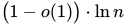
In low-frequency systems, Dinur et al. (2003) proved it is NP-hard to approximate set cover to better than $f-1-\epsilon$ . If the Unique games conjecture is true, this can be improved to $f-\epsilon$ as proven by Khot & Regev (2008).

Trevisan (2001) proves that set cover instances with sets of size at most $\Delta$ cannot be approximated to a factor better than $\ln \Delta -O(\ln \ln \Delta )$ unless P $=$ NP, thus making the approximation of $\ln \Delta +1$ of the greedy algorithm essentially tight in this case.

07Weighted set cover

The greedy algorithm for the weighted set cover problem directly generalizes the unweighted version. Given a universe ${\mathcal {U}}$ and a family ${\mathcal {S}}$ of subsets of ${\mathcal {U}}$ , where each set $S\in {\mathcal {S}}$ is assigned a non-negative weight (cost), the algorithm maintains the subset of elements that are not yet covered. Initially, all elements of ${\mathcal {U}}$ are uncovered. At each iteration, the algorithm selects a set $S\in {\mathcal {S}}$ that minimizes the ratio between its weight and the number of currently uncovered elements it contains. The selected set is added to the solution, and all elements contained in it are marked as covered. This process is repeated until all elements of ${\mathcal {U}}$ are covered. The greedy algorithm is known to produce a solution whose total weight is at most a factor of $H(n)$ times the optimal solution, where $H(n)$ denotes the $n$ -th harmonic number and $n=|{\mathcal {U}}|$ .

For low frequency systems, where every element is contained in at most $f$ sets, the deterministic LP rounding algorithm gets an $f$ -approximation. It starts with the optimal solution to the linear programming relaxation of the problem stated above. Sets whose fractional value exceeds $1/f$ are selected to form an integer solution.

The primal-dual algorithm for the set cover problem is an iterative method that constructs feasible solutions to both the primal and dual linear programs simultaneously. Starting with all dual variables set to zero, the algorithm repeatedly increases the dual variables corresponding to uncovered elements uniformly, until some set's dual constraint becomes tight (i.e., the sum of the dual variables for elements in the set equals its cost). This tight set is then added to the primal solution, covering the corresponding elements. The process continues until all elements are covered. The algorithm guarantees an approximation ratio of $f$ , where $f$ is the maximum number of sets that any element belongs to.

Randomized rounding is an approximation technique for the weighted set cover problem that uses the solution of the linear programming relaxation. Let ${x_{S}^{*}}$ be an optimal fractional solution to the LP relaxation. Each set $S\in {\mathcal {S}}$ is independently included in the cover with probability $x_{S}^{*}$ . By linearity of expectation, the expected cost of the chosen sets equals the LP optimum. The probability that any element remains uncovered can be made arbitrarily small by scaling probabilities or repeating the rounding. Using standard concentration bounds, this produces a feasible set cover whose expected cost is within an $O(\log n)$ factor of the optimal solution, where $n$ is the size of the universe.

References can be found in and.

Watch videos about Set cover problemExplainers and documentaries on YouTube (opens in a new tab)

Sources and credits

This article is adapted from the Wikipedia article “Set cover problem”, written by its contributors and licensed under CC BY-SA 4.0. Fathomly has changed the layout, removed citation markers, navigation and maintenance notices, and adjusted punctuation. This adapted version is shared under the same license. For references, see the original article.

Images, from Wikimedia Commons:

SetCover.svg by Jochen Burghardt, CC BY-SA 4.0
SetCoverGreedy.gif by Unknown author, Public domain

Fathomly is not affiliated with or endorsed by the Wikimedia Foundation. Spotted a problem? Tell us.