Encyclopedia

Autocorrelation

Correlation of a signal with a time-shifted copy of itself, as a function of shift

Wikipedia contributorsAdapted for Fathomly · View authors

18 min read
Source updated September 16, 2026

Autocorrelation, sometimes known as serial correlation in the discrete time case, measures the correlation of a signal with a delayed copy of itself. Essentially, it quantifies the similarity between observations of a random variable at different points in its domain (commonly, time). The analysis of autocorrelation is a mathematical tool for identifying repeating patterns or hidden periodicities within a signal obscured by noise. Autocorrelation is widely used in signal processing, time domain and time series analysis to understand the behavior of data over time.

Different fields of study define autocorrelation differently, and not all of these definitions are equivalent. In some fields, the term is used interchangeably with autocovariance.

Various time series models incorporate autocorrelation, such as unit root processes, trend-stationary processes, autoregressive processes, and moving average processes.

01Autocorrelation of stochastic processes

In statistics, the autocorrelation of a real or complex random process is the Pearson correlation between values of the process at different times, as a function of the two times or of the time lag. Let $\left\{X_{t}\right\}$ be a random process over time and $X_{t}$ be the random variable at time $t$ . ( $t$ may be an integer for a discrete-time process or a real number for a continuous-time process.) Then the definition of the autocorrelation function between times $t_{1}$ and $t_{2}$ is

$\operatorname {R} _{XX}(t_{1},t_{2})=\operatorname {E} \left[X_{t_{1}}{\overline {X}}_{t_{2}}\right]$

where $\operatorname {E}$ is the expected value operator and the bar represents complex conjugation. Note that the expectation may not be well defined.

Suppose that the process has mean $\mu _{t}$ and variance $\sigma _{t}^{2}$ at time $t$ , for each $t$ . Subtracting the mean before multiplication yields the auto-covariance function between times $t_{1}$ and $t_{2}$ :

${\begin{aligned}\operatorname {K} _{XX}(t_{1},t_{2})&=\operatorname {E} \left[(X_{t_{1}}-\mu _{t_{1}}){\overline {(X_{t_{2}}-\mu _{t_{2}})}}\right]\\&=\operatorname {E} \left[X_{t_{1}}{\overline {X}}_{t_{2}}\right]-\mu _{t_{1}}{\overline {\mu }}_{t_{2}}\\&=\operatorname {R} _{XX}(t_{1},t_{2})-\mu _{t_{1}}{\overline {\mu }}_{t_{2}}\end{aligned}}$

Note that this expression is not well defined for all-time series or processes, because the mean may not exist, or the variance may be zero (for a constant process) or infinite (for processes with distribution lacking well-behaved moments, such as certain types of power law).

Definition for wide-sense stationary stochastic process

If $\left\{X_{t}\right\}$ is a wide-sense stationary process then the mean $\mu$ and the variance $\sigma ^{2}$ are time-independent, and further the autocovariance function depends only on the lag between $t_{1}$ and $t_{2}$ : the autocovariance depends only on the time-distance between the pair of values but not on their position in time. This further implies that the autocovariance and autocorrelation can be expressed as a function of the time-lag, and that this would be an even function of the lag $\tau =t_{2}-t_{1}$ . This gives the more familiar forms for the autocorrelation function

$\operatorname {R} _{XX}(\tau )=\operatorname {E} \left[X_{t+\tau }{\overline {X}}_{t}\right]$

and the auto-covariance function:

${\begin{aligned}\operatorname {K} _{XX}(\tau )&=\operatorname {E} \left[(X_{t+\tau }-\mu ){\overline {(X_{t}-\mu )}}\right]\\&=\operatorname {E} \left[X_{t+\tau }{\overline {X}}_{t}\right]-\mu {\overline {\mu }}\\&=\operatorname {R} _{XX}(\tau )-\mu {\overline {\mu }}\end{aligned}}$

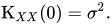
In particular, note that

$\operatorname {K} _{XX}(0)=\sigma ^{2}.$

Normalization

It is common practice in some disciplines (e.g. statistics and time series analysis) to normalize the autocovariance function to get a time-dependent Pearson correlation coefficient. However, in other disciplines (e.g. engineering) the normalization is usually dropped and the terms "autocorrelation" and "autocovariance" are used interchangeably.

The definition of the autocorrelation coefficient of a stochastic process is

${\begin{aligned}\rho _{XX}(t_{1},t_{2})&={\frac {\operatorname {K} _{XX}(t_{1},t_{2})}{\sigma _{t_{1}}\sigma _{t_{2}}}}\\&={\frac {\operatorname {E} \left[\left(X_{t_{1}}-\mu _{t_{1}}\right){\overline {\left(X_{t_{2}}-\mu _{t_{2}}\right)}}\right]}{\sigma _{t_{1}}\sigma _{t_{2}}}}.\end{aligned}}$

If the function $\rho _{XX}$ is well defined, its value must lie in the range $[-1,1]$ , with 1 indicating perfect correlation and −1 indicating perfect anti-correlation.

For a wide-sense stationary (WSS) process, the definition is

$\rho _{XX}(\tau )={\frac {\operatorname {K} _{XX}(\tau )}{\sigma ^{2}}}={\frac {\operatorname {E} \left[(X_{t+\tau }-\mu ){\overline {(X_{t}-\mu )}}\right]}{\sigma ^{2}}}.$

The normalization is important both because the interpretation of the autocorrelation as a correlation provides a scale-free measure of the strength of statistical dependence, and because the normalization has an effect on the statistical properties of the estimated autocorrelations.

Properties

Symmetry property

The fact that the autocorrelation function $\operatorname {R} _{XX}$ is an even function can be stated as $\operatorname {R} _{XX}(t_{1},t_{2})={\overline {\operatorname {R} _{XX}(t_{2},t_{1})}}$ respectively for a WSS process: $\operatorname {R} _{XX}(\tau )={\overline {\operatorname {R} _{XX}(-\tau )}}.$

Maximum at zero

For a WSS process: $\left|\operatorname {R} _{XX}(\tau )\right|\leq \operatorname {R} _{XX}(0)$ Notice that $\operatorname {R} _{XX}(0)$ is always real.

Cauchy-Schwarz inequality

The Cauchy-Schwarz inequality, inequality for stochastic processes: $\left|\operatorname {R} _{XX}(t_{1},t_{2})\right|^{2}\leq \operatorname {E} \left[|X_{t_{1}}|^{2}\right]\operatorname {E} \left[|X_{t_{2}}|^{2}\right]$

Autocorrelation of white noise

The autocorrelation of a continuous-time white noise signal will have a strong peak (represented by a Dirac delta function) at $\tau =0$ and will be exactly $0$ for all other $\tau$ .

Wiener-Khinchin theorem

The Wiener-Khinchin theorem relates the autocorrelation function $\operatorname {R} _{XX}$ to the power spectral density $S_{XX}$ via the Fourier transform:

${\begin{aligned}\operatorname {R} _{XX}(\tau )&=\int _{-\infty }^{\infty }S_{XX}(\omega )e^{i\omega \tau }\,{\rm {d}}\omega \\[1ex]S_{XX}(\omega )&=\int _{-\infty }^{\infty }\operatorname {R} _{XX}(\tau )e^{-i\omega \tau }\,{\rm {d}}\tau .\end{aligned}}$

For real-valued functions, the symmetric autocorrelation function has a real symmetric transform, so the Wiener-Khinchin theorem can be re-expressed in terms of real cosines only:

${\begin{aligned}\operatorname {R} _{XX}(\tau )&=\int _{-\infty }^{\infty }S_{XX}(\omega )\cos(\omega \tau )\,{\rm {d}}\omega \\[1ex]S_{XX}(\omega )&=\int _{-\infty }^{\infty }\operatorname {R} _{XX}(\tau )\cos(\omega \tau )\,{\rm {d}}\tau .\end{aligned}}$

02Autocorrelation of random vectors

The (potentially time-dependent) autocorrelation matrix (also called second moment) of a (potentially time-dependent) random vector $\mathbf {X} =(X_{1},\ldots ,X_{n})^{\rm {T}}$ is an $n\times n$ matrix containing as elements the autocorrelations of all pairs of elements of the random vector $\mathbf {X}$ . The autocorrelation matrix is used in various digital signal processing algorithms.

For a random vector $\mathbf {X} =(X_{1},\ldots ,X_{n})^{\rm {T}}$ containing random elements whose expected value and variance exist, the autocorrelation matrix is defined by

$\operatorname {R} _{\mathbf {X} \mathbf {X} }\triangleq \ \operatorname {E} \left[\mathbf {X} \mathbf {X} ^{\rm {T}}\right]$

where ${}^{\rm {T}}$ denotes transposition of the vector.

$\operatorname {R} _{\mathbf {X} \mathbf {X} }$ is a matrix of dimensions $n\times n$ :

$\operatorname {R} _{\mathbf {X} \mathbf {X} }={\begin{bmatrix}\operatorname {E} [X_{1}X_{1}]&\operatorname {E} [X_{1}X_{2}]&\cdots &\operatorname {E} [X_{1}X_{n}]\\\\\operatorname {E} [X_{2}X_{1}]&\operatorname {E} [X_{2}X_{2}]&\cdots &\operatorname {E} [X_{2}X_{n}]\\\\\vdots &\vdots &\ddots &\vdots \\\\\operatorname {E} [X_{n}X_{1}]&\operatorname {E} [X_{n}X_{2}]&\cdots &\operatorname {E} [X_{n}X_{n}]\end{bmatrix}}$

For example, if $\mathbf {X} =\left(X_{1},X_{2},X_{3}\right)^{\rm {T}}$ is a random vector, then $\operatorname {R} _{\mathbf {X} \mathbf {X} }$ is a $3\times 3$ matrix whose $(i,j)$ -th entry is $\operatorname {E} [X_{i}X_{j}]$ .

If $\mathbf {Z}$ is a complex random vector, the autocorrelation matrix is instead defined by

$\operatorname {R} _{\mathbf {Z} \mathbf {Z} }\triangleq \ \operatorname {E} [\mathbf {Z} \mathbf {Z} ^{\rm {H}}].$

Here ${}^{\rm {H}}$ denotes Hermitian transpose.

Properties of the autocorrelation matrix

The autocorrelation matrix is a Hermitian matrix for complex random vectors and a symmetric matrix for real random vectors.
The autocorrelation matrix is a positive semidefinite matrix, i.e. $\mathbf {a} ^{\mathrm {T} }\operatorname {R} _{\mathbf {X} \mathbf {X} }\mathbf {a} \geq 0\quad {\text{for all }}\mathbf {a} \in \mathbb {R} ^{n}$ for a real random vector, and respectively $\mathbf {a} ^{\mathrm {H} }\operatorname {R} _{\mathbf {Z} \mathbf {Z} }\mathbf {a} \geq 0\quad {\text{for all }}\mathbf {a} \in \mathbb {C} ^{n}$ in case of a complex random vector.
All eigenvalues of the autocorrelation matrix are real and non-negative.
The auto-covariance matrix is related to the autocorrelation matrix as follows: ${\begin{aligned}\operatorname {K} _{\mathbf {X} \mathbf {X} }&=\operatorname {E} \left[(\mathbf {X} -\operatorname {E} [\mathbf {X} ])(\mathbf {X} -\operatorname {E} [\mathbf {X} ])^{\rm {T}}\right]\\&=\operatorname {R} _{\mathbf {X} \mathbf {X} }-\operatorname {E} [\mathbf {X} ]\operatorname {E} [\mathbf {X} ]^{\rm {T}}\end{aligned}}$ Respectively for complex random vectors: ${\begin{aligned}\operatorname {K} _{\mathbf {Z} \mathbf {Z} }&=\operatorname {E} \left[(\mathbf {Z} -\operatorname {E} [\mathbf {Z} ])(\mathbf {Z} -\operatorname {E} [\mathbf {Z} ])^{\rm {H}}\right]\\&=\operatorname {R} _{\mathbf {Z} \mathbf {Z} }-\operatorname {E} [\mathbf {Z} ]\operatorname {E} [\mathbf {Z} ]^{\rm {H}}\end{aligned}}$

03Autocorrelation of deterministic signals

In signal processing, the above definition is often used without the normalization, that is, without subtracting the mean and dividing by the variance. When the autocorrelation function is normalized by mean and variance, it is sometimes referred to as the autocorrelation coefficient or autocovariance function.

Autocorrelation of continuous-time signal

Given a signal $f(t)$ , the continuous autocorrelation $R_{ff}(\tau )$ is most often defined as the continuous cross-correlation integral of $f(t)$ with itself, at lag $\tau$ .

$R_{ff}(\tau )=\int _{-\infty }^{\infty }f(t+\tau ){\overline {f(t)}}\,{\rm {d}}t=\int _{-\infty }^{\infty }f(t){\overline {f(t-\tau )}}\,{\rm {d}}t$

where ${\overline {f(t)}}$ represents the complex conjugate of $f(t)$ . Note that the parameter $t$ in the integral is a dummy variable and is only necessary to calculate the integral. It has no specific meaning.

Autocorrelation of discrete-time signal

The discrete autocorrelation $R$ at lag $\ell$ for a discrete-time signal $y(n)$ is

$R_{yy}(\ell )=\sum _{n\in Z}y(n)\,{\overline {y(n-\ell )}}$

The above definitions work for signals that are square integrable, or square summable, that is, of finite energy. Signals that "last forever" are treated instead as random processes, in which case different definitions are needed, based on expected values. For wide-sense-stationary random processes, the autocorrelations are defined as

${\begin{aligned}R_{ff}(\tau )&=\operatorname {E} \left[f(t){\overline {f(t-\tau )}}\right]\\R_{yy}(\ell )&=\operatorname {E} \left[y(n)\,{\overline {y(n-\ell )}}\right].\end{aligned}}$

For processes that are not stationary, these will also be functions of $t$ , or $n$ .

For processes that are also ergodic, the expectation can be replaced by the limit of a time average. The autocorrelation of an ergodic process is sometimes defined as or equated to

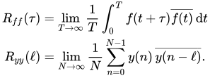
${\begin{aligned}R_{ff}(\tau )&=\lim _{T\rightarrow \infty }{\frac {1}{T}}\int _{0}^{T}f(t+\tau ){\overline {f(t)}}\,{\rm {d}}t\\R_{yy}(\ell )&=\lim _{N\rightarrow \infty }{\frac {1}{N}}\sum _{n=0}^{N-1}y(n)\,{\overline {y(n-\ell )}}.\end{aligned}}$

These definitions have the advantage that they give sensible well-defined single-parameter results for periodic functions, even when those functions are not the output of stationary ergodic processes.

Alternatively, signals that last forever can be treated by a short-time autocorrelation function analysis, using finite time integrals. (See short-time Fourier transform for a related process.)

Definition for periodic signals

If $f$ is a continuous periodic function of period $T$ , the integration from $-\infty$ to $\infty$ is replaced by integration over any interval $[t_{0},t_{0}+T]$ of length $T$ :

$R_{ff}(\tau )\triangleq \int _{t_{0}}^{t_{0}+T}f(t+\tau ){\overline {f(t)}}\,dt$

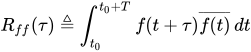
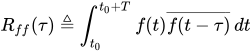
which is equivalent to

$R_{ff}(\tau )\triangleq \int _{t_{0}}^{t_{0}+T}f(t){\overline {f(t-\tau )}}\,dt$

Properties

In the following, we will describe properties of one-dimensional autocorrelations only, since most properties are easily transferred from the one-dimensional case to the multi-dimensional cases. These properties hold for wide-sense stationary processes.

A fundamental property of the autocorrelation is symmetry, , which is easy to prove from the definition. In the continuous case,
- the autocorrelation is an even function $R_{ff}(-\tau )=R_{ff}(\tau )$ when $f$ is a real function, and
- the autocorrelation is a Hermitian function $R_{ff}(-\tau )=R_{ff}^{*}(\tau )$ when $f$ is a complex function.
The continuous autocorrelation function reaches its peak at the origin, where it takes a real value, i.e. for any delay $\tau$ , $|R_{ff}(\tau )|\leq R_{ff}(0)$ . This is a consequence of the rearrangement inequality. The same result holds in the discrete case.
The autocorrelation of a periodic function is, itself, periodic with the same period.
The autocorrelation of the sum of two completely uncorrelated functions (the cross-correlation is zero for all $\tau$ ) is the sum of the autocorrelations of each function separately.
Since autocorrelation is a specific type of cross-correlation, it maintains all the properties of cross-correlation.
By using the symbol $*$ to represent convolution and $g_{-1}$ is a function which manipulates the function $f$ and is defined as $g_{-1}(f)(t)=f(-t)$ , the definition for $R_{ff}(\tau )$ may be written as: $R_{ff}(\tau )=(f*g_{-1}({\overline {f}}))(\tau )$

04Multi-dimensional autocorrelation

Multi-dimensional autocorrelation is defined similarly. For example, in three dimensions the autocorrelation of a square-summable discrete signal would be

$R(j,k,\ell )=\sum _{n,q,r}x_{n,q,r}\,{\overline {x}}_{n-j,q-k,r-\ell }.$

When mean values are subtracted from signals before computing an autocorrelation function, the resulting function is usually called an auto-covariance function.

05Efficient computation

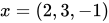
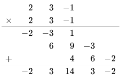
For data expressed as a discrete sequence, it is frequently necessary to compute the autocorrelation with high computational efficiency. A brute force method based on the signal processing definition ${\textstyle R_{xx}(j)=\sum _{n}x_{n}\,{\overline {x}}_{n-j}$ can be used when the signal size is small. For example, to calculate the autocorrelation of the real signal sequence $x=(2,3,-1)$ (i.e. $x_{0}=2,x_{1}=3,x_{2}=-1$ , and $x_{i}=0$ for all other values of i) by hand, we first recognize that the definition just given is the same as the "usual" multiplication, but with right shifts, where each vertical addition gives the autocorrelation for particular lag values: ${\begin{array}{rrrrrr}&2&3&-1\\\times &2&3&-1\\\hline &-2&-3&1\\&&6&9&-3\\+&&&4&6&-2\\\hline &-2&3&14&3&-2\end{array}}$

Thus the required autocorrelation sequence is $R_{xx}=(-2,3,14,3,-2)$ , where $R_{xx}(0)=14,$ $R_{xx}(-1)=R_{xx}(1)=3,$ and $R_{xx}(-2)=R_{xx}(2)=-2,$ the autocorrelation for other lag values being zero. In this calculation we do not perform the carry-over operation during addition as is usual in normal multiplication. Note that we can halve the number of operations required by exploiting the inherent symmetry of the autocorrelation. If the signal happens to be periodic, i.e. $x=(\ldots ,2,3,-1,2,3,-1,\ldots ),$ then we get a circular autocorrelation (similar to circular convolution) where the left and right tails of the previous autocorrelation sequence will overlap and give $R_{xx}=(\ldots ,14,1,1,14,1,1,\ldots )$ which has the same period as the signal sequence $x.$ The procedure can be regarded as an application of the convolution property of Z-transform of a discrete signal.

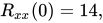
While the brute force algorithm is order n², several efficient algorithms exist which can compute the autocorrelation in order n log(n). For example, the Wiener-Khinchin theorem allows computing the autocorrelation from the raw data X(t) with two fast Fourier transforms (FFT):

${\begin{aligned}F_{R}(f)&=\operatorname {FFT} [X(t)]\\S(f)&=F_{R}(f)F_{R}^{*}(f)\\R(\tau )&=\operatorname {IFFT} [S(f)]\end{aligned}}$

where IFFT denotes the inverse fast Fourier transform. The asterisk denotes complex conjugate.

Alternatively, a multiple τ correlation can be performed by using brute force calculation for low τ values, and then progressively binning the X(t) data with a logarithmic density to compute higher values, resulting in the same n log(n) efficiency, but with lower memory requirements.

06Estimation

For a discrete process with known mean and variance for which we observe $n$ observations $\{X_{1},\,X_{2},\,\ldots ,\,X_{n}\}$ , an estimate of the autocorrelation coefficient may be obtained as

${\hat {R}}(k)={\frac {1}{(n-k)\sigma ^{2}}}\sum _{t=1}^{n-k}(X_{t}-\mu )(X_{t+k}-\mu )$

for any positive integer $k<n$ . When the true mean $\mu$ and variance $\sigma ^{2}$ are known, this estimate is unbiased. If the true mean and variance of the process are not known there are several possibilities:

If $\mu$ and $\sigma ^{2}$ are replaced by the standard formulae for sample mean and sample variance, then this is a biased estimate.
A periodogram-based estimate replaces $n-k$ in the above formula with $n$ . This estimate is always biased; however, it usually has a smaller mean squared error.
Other possibilities derive from treating the two portions of data $\{X_{1},\,X_{2},\,\ldots ,\,X_{n-k}\}$ and $\{X_{k+1},\,X_{k+2},\,\ldots ,\,X_{n}\}$ separately and calculating separate sample means and/or sample variances for use in defining the estimate.

The advantage of estimates of the last type is that the set of estimated autocorrelations, as a function of $k$ , then form a function which is a valid autocorrelation in the sense that it is possible to define a theoretical process having exactly that autocorrelation. Other estimates can suffer from the problem that, if they are used to calculate the variance of a linear combination of the $X$ 's, the variance calculated may turn out to be negative.

07Hassani −1/2 theorem

In time series analysis, the Hassani −1/2 theorem is a finite-sample identity concerning the conventional sample-mean-corrected estimator of the sample autocorrelation function (ACF). It states that, when the sample autocorrelations of a finite time series are calculated using a common normalization over all available positive lags, their sum is fixed at $-1/2$ .

For observations $x_{1},\ldots ,x_{T}$ , let

$z_{t}=x_{t}-{\bar {x}},$

where ${\bar {x}}$ is the sample mean. With the commonly used estimator

${\hat {\rho }}(h)={\frac {\displaystyle \sum _{t=1}^{T-h}z_{t}z_{t+h}}{\displaystyle \sum _{t=1}^{T}z_{t}^{2}}},\qquad h=1,\ldots ,T-1,$

the theorem gives

$\sum _{h=1}^{T-1}{\hat {\rho }}(h)=-{\frac {1}{2}},$

provided that the sample is non-constant so that the denominator is non-zero.

Although the original result was formulated in the context of stationary time series, the equality arises from an algebraic constraint produced by centering observations using the sample mean. It is therefore principally a finite-sample property of this particular ACF estimator rather than a statement about the dependence structure of the stochastic process generating the observations.

Algebraic basis

The identity follows from the fact that the centered observations satisfy

$\sum _{t=1}^{T}z_{t}=0.$

Squaring this relation gives

$0=\left(\sum _{t=1}^{T}z_{t}\right)^{2}=\sum _{t=1}^{T}z_{t}^{2}+2\sum _{1\leq t<s\leq T}z_{t}z_{s}.$

The second term contains every pairwise product of observations at positive separations. Grouping these products according to their lag yields

$\sum _{h=1}^{T-1}\sum _{t=1}^{T-h}z_{t}z_{t+h}=-{\frac {1}{2}}\sum _{t=1}^{T}z_{t}^{2}.$

Dividing both sides by $\sum _{t=1}^{T}z_{t}^{2}$ gives the −1/2 identity.

This derivation also demonstrates why the result does not imply that the theoretical autocorrelations of the underlying process sum to −1/2. The restriction arises because the same data are used both to estimate the sample mean and to construct all of the empirical autocorrelations.

Related finite-sample effects arising from estimation of an unknown mean had previously been discussed by Percival, who showed that conventional estimators of variance and autocovariance can possess unintuitive properties when the population mean is replaced by the sample mean.

Statistical interpretation

A consequence of the theorem is that the complete vector of sample autocorrelations,

$({\hat {\rho }}(1),\ldots ,{\hat {\rho }}(T-1)),$

is subject to an exact linear constraint. The sample autocorrelations at different lags therefore cannot be mutually independent when the complete collection of lags is considered.

This observation is relevant to standard large-sample approximations in time-series analysis. For certain processes, sample autocorrelations at a fixed and relatively small number of lags may be approximately normally distributed and asymptotically uncorrelated. The −1/2 theorem does not contradict such fixed-lag asymptotic results. Instead, it shows that these approximations cannot be extended indiscriminately to the entire set of $T-1$ sample autocorrelations, because the full collection satisfies the exact finite-sample constraint.

The theorem also implies that positive empirical correlations at some lags must be offset by negative contributions at other lags when all positive lags are included. Consequently, the unrestricted sum of sample autocorrelations cannot be interpreted directly as an empirical measure of the overall amount or direction of serial dependence.

Relation to long-memory processes

The distinction between theoretical and sample autocorrelations is particularly important in the study of long-memory processes. A common theoretical characterization of long memory is based on a slowly decaying autocorrelation function whose infinite sum does not converge absolutely, or may diverge.

For a finite sample, however, the sum of the conventionally estimated autocorrelations over all available positive lags remains −1/2, irrespective of whether the underlying process is theoretically short-memory or long-memory. Hassani, Leonenko and Patterson therefore argued that the full sum of sample autocorrelations cannot itself be used as a consistent empirical diagnostic for long-range dependence.

This does not imply that sample autocorrelations contain no information about long memory. Rather, inference generally depends on the rate of decay, selected ranges of lags, spectral behaviour near frequency zero, or dedicated estimators of long-memory parameters instead of the unrestricted sum across every available lag.

Diagnostic testing and the Ljung-Box statistic

The theorem has also been examined in connection with residual diagnostics and portmanteau tests. The Ljung-Box test, for example, is based on a weighted sum of squared sample autocorrelations over a specified number of lags rather than on their simple signed sum.

Hassani and Yeganegi investigated how results of the Ljung-Box procedure can depend on the number of included lags and used the −1/2 identity as motivation for studying the collective behaviour of sample autocorrelations.

Their analysis emphasized that diagnostic conclusions may change with the truncation lag used in a portmanteau statistic and that finite-sample dependence among estimated autocorrelations should be distinguished from asymptotic approximations applying to a fixed number of lags.

Subsequent work has similarly examined the behaviour of sample ACFs for white-noise and fitted-model residuals and has questioned whether standard normal approximations remain satisfactory when increasingly large sets of lags are considered.

Model identification

Sample ACFs are widely used for identifying time-series models, particularly moving-average (MA) processes, for which the theoretical ACF becomes zero beyond the model order. In finite samples, however, estimated autocorrelations fluctuate around their theoretical values.

Recent research has used the −1/2 theorem to investigate the joint behaviour and distribution of sample ACFs in white-noise and MA processes. Hassani and co-authors reported departures from simple independent-normal approximations when a sufficiently large range of sample autocorrelations is considered.

Royer-Carenzi and Hassani subsequently examined the implications for identifying MA( $q$ ) and ARMA( $p,q$ ) models, including procedures based on the ACF and extended autocorrelation function. Their simulations indicated that conventional identification methods remain useful for sufficiently long samples but may be less reliable in particular parameter configurations, motivating the use of additional diagnostics and predictive comparisons.

Short-memory processes

The −1/2 identity has also been discussed in relation to empirical definitions of short-memory processes. Some definitions characterize short memory through summability or rapid decay of theoretical autocorrelations. Because the complete finite-sample ACF sum is predetermined, directly transferring such a theoretical summability criterion to the unrestricted empirical ACF can be problematic.

Hassani and co-authors revisited commonly used definitions of short memory and argued that empirical identification should distinguish properties of the underlying theoretical ACF from algebraic properties imposed on its finite-sample estimator.

Applications and related results

The −1/2 relation has appeared outside studies devoted specifically to sample-ACF methodology. For example, Di Crescenzo, Martinucci and Paraggio obtained autocorrelation structures for stationary interarrival times in a stochastic model of vessel arrivals and noted a −1/2 autocorrelation-sum relationship with reference to Hassani's earlier result.

Computational implementations of the sum-of-ACF quantity have also been made available in statistical software, including an R implementation for calculating the complete sample-ACF sum.

Scope and limitations

The theorem depends on the definition of the sample ACF. In particular, the exact −1/2 equality applies to the conventional estimator in which the autocovariance numerator at each lag is normalized by the same lag-zero sum of squares after subtraction of the sample mean.

Alternative estimators may use different normalizations, bias corrections, known rather than estimated means, tapering, missing-data adjustments, or restrictions to a subset of lags. Such estimators need not satisfy the exact −1/2 identity.

The theorem should therefore not be interpreted as stating that

the theoretical ACF of every stochastic process sums to −1/2; every possible estimator of an ACF has this property; individual sample autocorrelations cannot be positive; standard fixed-lag asymptotic ACF theory is invalid; or ACF-based methods cannot be used for time-series identification.

Rather, it establishes an exact dependence constraint on the complete set of autocorrelations obtained from a particular finite-sample estimator.

Theoretical versus sample autocorrelation

The distinction between the theoretical and sample ACF is central to interpretation of the theorem. For a stationary stochastic process, the theoretical autocorrelation at lag $h$ is a population quantity,

$\rho (h)={\frac {\operatorname {Cov} (X_{t},X_{t+h})}{\operatorname {Var} (X_{t})}},$

and its behaviour depends on the underlying probability model. Its sum may be positive, negative, finite, divergent, or undefined depending on the process.

By contrast, ${\hat {\rho }}(h)$ is calculated from one finite realization. When the observations are centered using their own sample mean and the conventional common-denominator estimator is used, the complete finite-sample collection satisfies the deterministic −1/2 constraint. The theorem therefore illustrates a broader principle in time-series statistics: finite-sample estimators can possess structural properties that have no direct counterpart in the population quantity they estimate.

08Regression analysis

In regression analysis using time series data, autocorrelation in a variable of interest is typically modeled either with an autoregressive model (AR), a moving average model (MA), their combination as an autoregressive-moving-average model (ARMA), or an extension of the latter called an autoregressive integrated moving average model (ARIMA). With multiple interrelated data series, vector autoregression (VAR) or its extensions are used.

In ordinary least squares (OLS), the adequacy of a model specification can be checked in part by establishing whether there is autocorrelation of the regression residuals. Problematic autocorrelation of the errors, which themselves are unobserved, can generally be detected because it produces autocorrelation in the observable residuals. (Errors are also known as "error terms" in econometrics.) Autocorrelation of the errors violates the ordinary least squares assumption that the error terms are uncorrelated, meaning that the Gauss Markov theorem does not apply, and that OLS estimators are no longer the Best Linear Unbiased Estimators (BLUE). While it does not bias the OLS coefficient estimates, the standard errors tend to be underestimated (and the t-scores overestimated) when the autocorrelations of the errors at low lags are positive.

The traditional test for the presence of first-order autocorrelation is the Durbin-Watson statistic or, if the explanatory variables include a lagged dependent variable, Durbin's h statistic. The Durbin-Watson can be linearly mapped however to the Pearson correlation between values and their lags. A more flexible test, covering autocorrelation of higher orders and applicable whether or not the regressors include lags of the dependent variable, is the Breusch-Godfrey test. This involves an auxiliary regression, wherein the residuals obtained from estimating the model of interest are regressed on (a) the original regressors and (b) k lags of the residuals, where 'k' is the order of the test. The simplest version of the test statistic from this auxiliary regression is TR², where T is the sample size and R² is the coefficient of determination. Under the null hypothesis of no autocorrelation, this statistic is asymptotically distributed as $\chi ^{2}$ with k degrees of freedom.

Responses to nonzero autocorrelation include generalized least squares and the Newey-West HAC estimator (Heteroskedasticity and Autocorrelation Consistent).

In the estimation of a moving average model (MA), the autocorrelation function is used to determine the appropriate number of lagged error terms to be included. This is based on the fact that for an MA process of order q, we have $R(\tau )\neq 0$ , for $\tau =0,1,\ldots ,q$ , and $R(\tau )=0$ , for $\tau >q$ .

09Applications

Autocorrelation's ability to find repeating patterns in data yields many applications, including:

Autocorrelation analysis is used heavily in fluorescence correlation spectroscopy to provide quantitative insight into molecular-level diffusion and chemical reactions.
Another application of autocorrelation is the measurement of optical spectra and the measurement of very-short-duration light pulses produced by lasers, both using optical autocorrelators.
Autocorrelation is used to analyze dynamic light scattering data, which notably enables determination of the particle size distributions of nanometer-sized particles or micelles suspended in a fluid. A laser shining into the mixture produces a speckle pattern that results from the motion of the particles. Autocorrelation of the signal can be analyzed in terms of the diffusion of the particles. From this, knowing the viscosity of the fluid, the sizes of the particles can be calculated.
Utilized in the GPS system to correct for the propagation delay, or time shift, between the point of time at the transmission of the carrier signal at the satellites, and the point of time at the receiver on the ground. This is done by the receiver generating a replica signal of the 1,023-bit C/A (Coarse/Acquisition) code, and generating lines of code chips [-1,1] in packets of ten at a time, or 10,230 chips (1,023 × 10), shifting slightly as it goes along in order to accommodate for the doppler shift in the incoming satellite signal, until the receiver replica signal and the satellite signal codes match up.
The small-angle X-ray scattering intensity of a nanostructured system is the Fourier transform of the spatial autocorrelation function of the electron density.
In surface science and scanning probe microscopy, autocorrelation is used to establish a link between surface morphology and functional characteristics.
In optics, normalized autocorrelations and cross-correlations give the degree of coherence of an electromagnetic field.
In astronomy, autocorrelation can determine the frequency of pulsars.
In music, autocorrelation (when applied at time scales smaller than a second) is used as a pitch detection algorithm for both instrument tuners and "Auto Tune" (used as a distortion effect or to fix intonation). When applied at time scales larger than a second, autocorrelation can identify the musical beat, for example to determine tempo.
Autocorrelation in space rather than time, via the Patterson function, is used by X-ray diffractionists to help recover the "Fourier phase information" on atom positions not available through diffraction alone.
In statistics, spatial autocorrelation between sample locations also helps one estimate mean value uncertainties when sampling a heterogeneous population.
The SEQUEST algorithm for analyzing mass spectra makes use of autocorrelation in conjunction with cross-correlation to score the similarity of an observed spectrum to an idealized spectrum representing a peptide.
In astrophysics, autocorrelation is used to study and characterize the spatial distribution of galaxies in the universe and in multi-wavelength observations of low mass X-ray binaries.
In panel data, spatial autocorrelation refers to correlation of a variable with itself through space.
In analysis of Markov chain Monte Carlo data, autocorrelation must be taken into account for correct error determination.
In geosciences (specifically in geophysics) it can be used to compute an autocorrelation seismic attribute, out of a 3D seismic survey of the underground.
In medical ultrasound imaging, autocorrelation is used to visualize blood flow.
In intertemporal portfolio choice, the presence or absence of autocorrelation in an asset's rate of return can affect the optimal portion of the portfolio to hold in that asset.
In numerical relays, autocorrelation has been used to accurately measure power system frequency.

10Serial dependence

Serial dependence is closely linked to the notion of autocorrelation, but represents a distinct concept (see Correlation and dependence). In particular, it is possible to have serial dependence but no (linear) correlation. In some fields however, the two terms are used as synonyms.

A time series of a random variable has serial dependence if the value at some time $t$ in the series is statistically dependent on the value at another time $s$ . A series is serially independent if there is no dependence between any pair.

If a time series $\left\{X_{t}\right\}$ is stationary, then statistical dependence between the pair $(X_{t},X_{s})$ would imply that there is statistical dependence between all pairs of values at the same lag $\tau =s-t$ .

Watch videos about AutocorrelationExplainers and documentaries on YouTube (opens in a new tab)

Sources and credits

This article is adapted from the Wikipedia article “Autocorrelation”, written by its contributors and licensed under CC BY-SA 4.0. Fathomly has changed the layout, removed citation markers, navigation and maintenance notices, and adjusted punctuation. This adapted version is shared under the same license. For references, see the original article.

Images, from Wikimedia Commons:

Acf new.svg by Acf.svg: Jeremy Manning derivative work: Jrmanning (talk), CC BY-SA 3.0
Comparison convolution correlation.svg by Cmglee, CC BY-SA 3.0

Fathomly is not affiliated with or endorsed by the Wikimedia Foundation. Spotted a problem? Tell us.

Autocorrelation

01Autocorrelation of stochastic processes

Definition for wide-sense stationary stochastic process

Normalization

Properties

Symmetry property

Maximum at zero

Cauchy-Schwarz inequality

Autocorrelation of white noise

Wiener-Khinchin theorem

02Autocorrelation of random vectors

Properties of the autocorrelation matrix

03Autocorrelation of deterministic signals

Autocorrelation of continuous-time signal

Autocorrelation of discrete-time signal

Definition for periodic signals

Properties

04Multi-dimensional autocorrelation

05Efficient computation

06Estimation

07Hassani −1/2 theorem

Algebraic basis

Statistical interpretation

Relation to long-memory processes

Diagnostic testing and the Ljung-Box statistic

Model identification

Short-memory processes

Applications and related results

Scope and limitations

Theoretical versus sample autocorrelation

08Regression analysis

09Applications

10Serial dependence

Sources and credits

Related topics

Autocorrelation

Autocorrelation (words)

Autocorrelation technique