Encyclopedia

Remez algorithm

Algorithm to approximate functions

Wikipedia contributorsAdapted for Fathomly · View authors

4 min read
Source updated July 24, 2026

The Remez algorithm or Remez exchange algorithm, published by Evgeny Yakovlevich Remez in 1934, is an iterative algorithm used to find simple approximations to functions, specifically, approximations by functions in a Chebyshev space that are the best in the uniform norm L_∞ sense. It is sometimes referred to as Remes algorithm or Reme algorithm.

A typical example of a Chebyshev space is the subspace of Chebyshev polynomials of order n in the space of real continuous functions on an interval, C[a, b]. The polynomial of best approximation within a given subspace is defined to be the one that minimizes the maximum absolute difference between the polynomial and the function. In this case, the form of the solution is precised by the equioscillation theorem.

01Procedure

The Remez algorithm starts with the function $f$ to be approximated and a set $X$ of $n+2$ sample points $x_{1},x_{2},...,x_{n+2}$ in the approximation interval, usually the extrema of Chebyshev polynomial linearly mapped to the interval. The steps are:

Solve the linear system of equations

$b_{0}+b_{1}x_{i}+...+b_{n}x_{i}^{n}+(-1)^{i}E=f(x_{i})$ (where $i=1,2,...n+2$ ),

for the unknowns $b_{0},b_{1}...b_{n}$ and E.

Use the $b_{i}$ as coefficients to form a polynomial $P_{n}$ .
Find the set $M$ of points of local maximum error $|P_{n}(x)-f(x)|$ .
If the errors at every $m\in M$ are of equal magnitude and alternate in sign, then $P_{n}$ is the minimax approximation polynomial. If not, replace $X$ with $M$ and repeat the steps above.

The result is called the polynomial of best approximation or the minimax approximation algorithm.

A review of technicalities in implementing the Remez algorithm is given by W. Fraser.

Choice of initialization

The Chebyshev nodes are a common choice for the initial approximation because of their role in the theory of polynomial interpolation. For the initialization of the optimization problem for function f by the Lagrange interpolant L_n(f), it can be shown that this initial approximation is bounded by

$\lVert f-L_{n}(f)\rVert _{\infty }\leq (1+\lVert L_{n}\rVert _{\infty })\inf _{p\in P_{n}}\lVert f-p\rVert$

with the norm or Lebesgue constant of the Lagrange interpolation operator L_n of the nodes (t₁, ..., t_n + 1) being

$\lVert L_{n}\rVert _{\infty }={\overline {\Lambda }}_{n}(T)=\max _{-1\leq x\leq 1}\lambda _{n}(T;x),$

T being the zeros of the Chebyshev polynomials, and the Lebesgue functions being

$\lambda _{n}(T;x)=\sum _{j=1}^{n+1}\left|l_{j}(x)\right|,\quad l_{j}(x)=\prod _{\stackrel {i=1}{i\neq j}}^{n+1}{\frac {(x-t_{i})}{(t_{j}-t_{i})}}.$

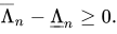
Theodore A. Kilgore, Carl de Boor, and Allan Pinkus proved that there exists a unique t_i for each L_n, although not known explicitly for (ordinary) polynomials. Similarly, ${\underline {\Lambda }}_{n}(T)=\min _{-1\leq x\leq 1}\lambda _{n}(T;x)$ , and the optimality of a choice of nodes can be expressed as ${\overline {\Lambda }}_{n}-{\underline {\Lambda }}_{n}\geq 0.$

For Chebyshev nodes, which provides a suboptimal, but analytically explicit choice, the asymptotic behavior is known as

${\overline {\Lambda }}_{n}(T)={\frac {2}{\pi }}\log(n+1)+{\frac {2}{\pi }}\left(\gamma +\log {\frac {8}{\pi }}\right)+\alpha _{n+1}$

(γ being the Euler-Mascheroni constant) with

$0<\alpha _{n}<{\frac {\pi }{72n^{2}}}$ for $n\geq 1,$

and upper bound

${\overline {\Lambda }}_{n}(T)\leq {\frac {2}{\pi }}\log(n+1)+1$

Lev Brutman obtained the bound for $n\geq 3$ , and ${\hat {T}}$ being the zeros of the expanded Chebyshev polynomials:

${\overline {\Lambda }}_{n}({\hat {T}})-{\underline {\Lambda }}_{n}({\hat {T}})<{\overline {\Lambda }}_{3}-{\frac {1}{6}}\cot {\frac {\pi }{8}}+{\frac {\pi }{64}}{\frac {1}{\sin ^{2}(3\pi /16)}}-{\frac {2}{\pi }}(\gamma -\log \pi )\approx 0.201.$

Rüdiger Günttner obtained from a sharper estimate for $n\geq 40$

${\overline {\Lambda }}_{n}({\hat {T}})-{\underline {\Lambda }}_{n}({\hat {T}})<0.0196.$

02Detailed discussion

This section provides more information on the steps outlined above. In this section, the index i runs from 0 to n+1.

Step 1: Given $x_{0},x_{1},...x_{n+1}$ , solve the linear system of n+2 equations

$b_{0}+b_{1}x_{i}+...+b_{n}x_{i}^{n}+(-1)^{i}E=f(x_{i})$ (where $i=0,1,...n+1$ ),

for the unknowns $b_{0},b_{1},...b_{n}$ and E.

It should be clear that $(-1)^{i}E$ in this equation makes sense only if the nodes $x_{0},...,x_{n+1}$ are ordered, either strictly increasing or strictly decreasing. Then this linear system has a unique solution. (As is well known, not every linear system has a solution.) Also, the solution can be obtained with only $O(n^{2})$ arithmetic operations while a standard solver from the library would take $O(n^{3})$ operations. Here is the simple proof:

Compute the standard n-th degree interpolant $p_{1}(x)$ to $f(x)$ at the first n+1 nodes and also the standard n-th degree interpolant $p_{2}(x)$ to the ordinates $(-1)^{i}$

$p_{1}(x_{i})=f(x_{i}),p_{2}(x_{i})=(-1)^{i},i=0,...,n.$

To this end, use each time Newton's interpolation formula with the divided differences of order $0,...,n$ and $O(n^{2})$ arithmetic operations.

The polynomial $p_{2}(x)$ has its i-th zero between $x_{i-1}$ and $x_{i},\ i=1,...,n$ , and thus no further zeroes between $x_{n}$ and $x_{n+1}$ : $p_{2}(x_{n})$ and $p_{2}(x_{n+1})$ have the same sign $(-1)^{n}$ .

The linear combination $p(x):=p_{1}(x)-p_{2}(x)\!\cdot \!E$ is also a polynomial of degree n and

$p(x_{i})=p_{1}(x_{i})-p_{2}(x_{i})\!\cdot \!E\ =\ f(x_{i})-(-1)^{i}E,\ \ \ \ i=0,\ldots ,n.$

This is the same as the equation above for $i=0,...,n$ and for any choice of E. The same equation for i = n+1 is

$p(x_{n+1})\ =\ p_{1}(x_{n+1})-p_{2}(x_{n+1})\!\cdot \!E\ =\ f(x_{n+1})-(-1)^{n+1}E$ and needs special reasoning: solved for the variable E, it is the definition of E:

$E\ :=\ {\frac {p_{1}(x_{n+1})-f(x_{n+1})}{p_{2}(x_{n+1})+(-1)^{n}}}.$

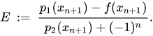
As mentioned above, the two terms in the denominator have same sign: E and thus $p(x)\equiv b_{0}+b_{1}x+\ldots +b_{n}x^{n}$ are always well-defined.

The error at the given n+2 ordered nodes is positive and negative in turn because

$p(x_{i})-f(x_{i})\ =\ -(-1)^{i}E,\ \ i=0,...,n\!+\!1.$

The equioscillation theorem states that under this condition no polynomial of degree n exists with error less than E. Indeed, if such a polynomial existed, call it ${\tilde {p}}(x)$ , then the difference $p(x)-{\tilde {p}}(x)=(p(x)-f(x))-({\tilde {p}}(x)-f(x))$ would still be positive/negative at the n+2 nodes $x_{i}$ and therefore have at least n+1 zeros which is impossible for a polynomial of degree n. Thus, this E is a lower bound for the minimum error which can be achieved with polynomials of degree n.

Step 2 changes the notation from $b_{0}+b_{1}x+...+b_{n}x^{n}$ to $p(x)$ .

Step 3 improves upon the input nodes $x_{0},...,x_{n+1}$ and their errors $\pm E$ as follows.

In each P-region, the current node $x_{i}$ is replaced with the local maximizer ${\bar {x}}_{i}$ and in each N-region $x_{i}$ is replaced with the local minimizer. (Expect ${\bar {x}}_{0}$ at A, the ${\bar {x}}_{i}$ near $x_{i}$ , and ${\bar {x}}_{n+1}$ at B.) No high precision is required here, the standard line search with a couple of quadratic fits should suffice. (See )

Let $z_{i}:=p({\bar {x}}_{i})-f({\bar {x}}_{i})$ . Each amplitude $|z_{i}|$ is greater than or equal to E. The Theorem of de La Vallée Poussin and its proof also apply to $z_{0},...,z_{n+1}$ with $\min\{|z_{i}|\}\geq E$ as the new lower bound for the best error possible with polynomials of degree n.

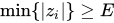
Moreover, $\max\{|z_{i}|\}$ comes in handy as an obvious upper bound for that best possible error.

Step 4: With $\min \,\{|z_{i}|\}$ and $\max \,\{|z_{i}|\}$ as lower and upper bound for the best possible approximation error, one has a reliable stopping criterion: repeat the steps until $\max\{|z_{i}|\}-\min\{|z_{i}|\}$ is sufficiently small or no longer decreases. These bounds indicate the progress.

03Variants

Some modifications of the algorithm are present on the literature. These include:

Replacing more than one sample point with the locations of nearby maximum absolute differences.
Replacing all of the sample points with in a single iteration with the locations of all, alternating sign, maximum differences.
Using the relative error to measure the difference between the approximation and the function, especially if the approximation will be used to compute the function on a computer which uses floating point arithmetic;
Including zero-error point constraints.
The Fraser-Hart variant, used to determine the best rational Chebyshev approximation.

Watch videos about Remez algorithmExplainers and documentaries on YouTube (opens in a new tab)

Sources and credits

This article is adapted from the Wikipedia article “Remez algorithm”, written by its contributors and licensed under CC BY-SA 4.0. Fathomly has changed the layout, removed citation markers, navigation and maintenance notices, and adjusted punctuation. This adapted version is shared under the same license. For references, see the original article.

Fathomly is not affiliated with or endorsed by the Wikimedia Foundation. Spotted a problem? Tell us.

Remez algorithm

01Procedure

Choice of initialization

02Detailed discussion

03Variants

Sources and credits

Related topics

Hadamard's lemma

Laurent series

Padé approximant