Radial basis function kernel
Machine learning kernel function
In machine learning, the radial basis function kernel, or RBF kernel, is a popular kernel function used in various kernelized learning algorithms. In particular, it is commonly used in support vector machine classification.
The RBF kernel on two samples 
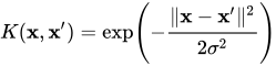



Since the value of the RBF kernel decreases with distance and ranges between zero (in the infinite-distance limit) and one (when x = x'), it has a ready interpretation as a similarity measure.
The feature space of the kernel has an infinite number of dimensions; for 
![{\begin{alignedat}{2}\exp \left(-{\frac {1}{2}}\|\mathbf {x} -\mathbf {x'} \|^{2}\right)&=\exp \left({\frac {2}{2}}\mathbf {x} ^{\top }\mathbf {x'} -{\frac {1}{2}}\|\mathbf {x} \|^{2}-{\frac {1}{2}}\|\mathbf {x'} \|^{2}\right)\\[5pt]&=\exp \left(\mathbf {x} ^{\top }\mathbf {x'} \right)\exp \left(-{\frac {1}{2}}\|\mathbf {x} \|^{2}\right)\exp \left(-{\frac {1}{2}}\|\mathbf {x'} \|^{2}\right)\\[5pt]&=\sum _{j=0}^{\infty }{\frac {(\mathbf {x} ^{\top }\mathbf {x'} )^{j}}{j!}}\exp \left(-{\frac {1}{2}}\|\mathbf {x} \|^{2}\right)\exp \left(-{\frac {1}{2}}\|\mathbf {x'} \|^{2}\right)\\[5pt]&=\sum _{j=0}^{\infty }\quad \sum _{n_{1}+n_{2}+\dots +n_{k}=j}\exp \left(-{\frac {1}{2}}\|\mathbf {x} \|^{2}\right){\frac {x_{1}^{n_{1}}\cdots x_{k}^{n_{k}}}{\sqrt {n_{1}!\cdots n_{k}!}}}\exp \left(-{\frac {1}{2}}\|\mathbf {x'} \|^{2}\right){\frac {{x'}_{1}^{n_{1}}\cdots {x'}_{k}^{n_{k}}}{\sqrt {n_{1}!\cdots n_{k}!}}}\\[5pt]&=\langle \varphi (\mathbf {x} ),\varphi (\mathbf {x'} )\rangle \end{alignedat}}](https://wikimedia.org/api/rest_v1/media/math/render/svg/c42c51e11b675698e01290de18306bcb7acc613f)



01Approximations
Because support vector machines and other models employing the kernel trick do not scale well to large numbers of training samples or large numbers of features in the input space, several approximations to the RBF kernel (and similar kernels) have been introduced. Typically, these take the form of a function z that maps a single vector to a vector of higher dimensionality, approximating the kernel:

where 
Fourier random features
One way to construct such a z is to randomly sample from the Fourier transformation of the kernel![\varphi (x)={\frac {1}{\sqrt {D}}}[\cos \langle w_{1},x\rangle ,\sin \langle w_{1},x\rangle ,\ldots ,\cos \langle w_{D},x\rangle ,\sin \langle w_{D},x\rangle ]^{T}](https://wikimedia.org/api/rest_v1/media/math/render/svg/1ebebe5193c52efc25a749492cf0269cd44e7f0d)


Theorem:
![\operatorname {E} [\langle \varphi (x),\varphi (y)\rangle ]=e^{\|x-y\|^{2}/(2\sigma ^{2})}.](https://wikimedia.org/api/rest_v1/media/math/render/svg/e2cc6c1d5eada384ef6b1f2a462dfa2089921bfb)
Proof: It suffices to prove the case of 

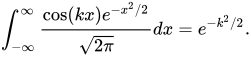
Theorem: ![\operatorname {Var} [\langle \varphi (x),\varphi (y)\rangle ]=O(D^{-1})](https://wikimedia.org/api/rest_v1/media/math/render/svg/e8ab3082dbba4fa920eee2c462249655c7908dc0)
Nyström method
Another approach uses the Nyström method to approximate the eigendecomposition of the Gram matrix K, using only a random sample of the training set.
Sources and credits
This article is adapted from the Wikipedia article “Radial basis function kernel”, written by its contributors and licensed under CC BY-SA 4.0. Fathomly has changed the layout, removed citation markers, navigation and maintenance notices, and adjusted punctuation. This adapted version is shared under the same license. For references, see the original article.
Fathomly is not affiliated with or endorsed by the Wikimedia Foundation. Spotted a problem? Tell us.
