PROPT

PROPT is a combined modeling, compilation and solver engine, built upon the TomSym modeling class, for generation of highly complex optimal control problems. PROPT uses a pseudospectral Collocation method (with Gauss or Chebyshev points) for solving optimal control problems. This means that the solution takes the form of a Polynomial, and this polynomial satisfies the DAE and the path constraints at the collocation points.

In general PROPT has the following main functions:

• Computation of the constant matrices used for the differentiation and integration of the polynomials used to approximate the solution to the Trajectory optimization problem.
• Source transformation to turn user-supplied expressions into MATLAB code for the cost function and constraint function that are passed to a Nonlinear programming solver in TOMLAB. The source transformation package TomSym automatically generates first and second order derivatives.
• Functionality for plotting and computing a variety of information for the solution to the problem.
• Automatic detection of the following:
  • Linear and quadratic objective.
  • Simple bounds, linear and nonlinear constraints.
  • Non-optimized expressions.
• Integrated support for non-smooth (hybrid) optimal control problems.
• Module for automatic scaling of difficult space related problem.
• Support for binary and integer variables, controls or states.

The PROPT system uses the TomSym symbolic source transformation engine to model optimal control problems. It is possible to define independent variables, dependent functions, scalars and constant parameters:

toms tf toms t p = tomPhase('p', t, 0, tf, 30); x0 = {tf == 20}; cbox = {10 <= tf <= 40}; toms z1 cbox = {cbox; 0 <= z1 <= 500}; x0 = {x0; z1 == 0}; ki0 = [1e3; 1e7; 10; 1e-3];

States and controls

States and controls only differ in the sense that states need be continuous between phases.

tomStates x1 x0 = {icollocate({x1 == 0})}; tomControls u1 cbox = {-2 <= collocate(u1) <= 1}; x0 = {x0; collocate(u1 == -0.01)};

Boundary, path, event and integral constraints

A variety of boundary, path, event and integral constraints are shown below:

cbnd = initial(x1 == 1); % Starting point for x1 cbnd = final(x1 == 1); % End point for x1 cbnd = final(x2 == 2); % End point for x2 pathc = collocate(x3 >= 0.5); % Path constraint for x3 intc = {integrate(x2) == 1}; % Integral constraint for x2 cbnd = final(x3 >= 0.5); % Final event constraint for x3 cbnd = initial(x1 <= 2.0); % Initial event constraint x1

Van der Pol Oscillator

Minimize:

Subject to:

To solve the problem with PROPT the following code can be used (with 60 collocation points):

toms t p = tomPhase('p', t, 0, 5, 60); setPhase(p); tomStates x1 x2 x3 tomControls u % Initial guess x0 = {icollocate({x1 == 0; x2 == 1; x3 == 0}) collocate(u == -0.01)}; % Box constraints cbox = {-10 <= icollocate(x1) <= 10 -10 <= icollocate(x2) <= 10 -10 <= icollocate(x3) <= 10 -0.3 <= collocate(u) <= 1}; % Boundary constraints cbnd = initial({x1 == 0; x2 == 1; x3 == 0}); % ODEs and path constraints ceq = collocate({dot(x1) == (1-x2.^2).*x1-x2+u dot(x2) == x1; dot(x3) == x1.^2+x2.^2+u.^2}); % Objective objective = final(x3); % Solve the problem options = struct; options.name = 'Van Der Pol'; solution = ezsolve(objective, {cbox, cbnd, ceq}, x0, options);

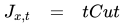
One-dimensional rocket with free end time and undetermined phase shift

Minimize:

Subject to:

The problem is solved with PROPT by creating two phases and connecting them:

toms t toms tCut tp2 p1 = tomPhase('p1', t, 0, tCut, 20); p2 = tomPhase('p2', t, tCut, tp2, 20); tf = tCut+tp2; x1p1 = tomState(p1,'x1p1'); x2p1 = tomState(p1,'x2p1'); x1p2 = tomState(p2,'x1p2'); x2p2 = tomState(p2,'x2p2'); % Initial guess x0 = {tCut==10 tf==15 icollocate(p1,{x1p1 == 50*tCut/10;x2p1 == 0;}) icollocate(p2,{x1p2 == 50+50*t/100;x2p2 == 0;})}; % Box constraints cbox = { 1 <= tCut <= tf-0.00001 tf <= 100 0 <= icollocate(p1,x1p1) 0 <= icollocate(p1,x2p1) 0 <= icollocate(p2,x1p2) 0 <= icollocate(p2,x2p2)}; % Boundary constraints cbnd = {initial(p1,{x1p1 == 0;x2p1 == 0;}) final(p2,x1p2 == 100)}; % ODEs and path constraints a = 2; g = 1; ceq = {collocate(p1,{ dot(p1,x1p1) == x2p1 dot(p1,x2p1) == a-g}) collocate(p2,{ dot(p2,x1p2) == x2p2 dot(p2,x2p2) == -g})}; % Objective objective = tCut; % Link phase link = {final(p1,x1p1) == initial(p2,x1p2) final(p1,x2p1) == initial(p2,x2p2)}; %% Solve the problem options = struct; options.name = 'One Dim Rocket'; constr = {cbox, cbnd, ceq, link}; solution = ezsolve(objective, constr, x0, options);

Parameter estimation problem

Minimize:

Subject to:

In the code below the problem is solved with a fine grid (10 collocation points). This solution is subsequently fine-tuned using 40 collocation points:

toms t p1 p2 x1meas = [0.264;0.594;0.801;0.959]; tmeas = [1;2;3;5]; % Box constraints cbox = {-1.5 <= p1 <= 1.5 -1.5 <= p2 <= 1.5}; %% Solve the problem, using a successively larger number collocation points for n=[10 40] p = tomPhase('p', t, 0, 6, n); setPhase(p); tomStates x1 x2 % Initial guess if n == 10 x0 = {p1 == 0; p2 == 0}; else x0 = {p1 == p1opt; p2 == p2opt icollocate({x1 == x1opt; x2 == x2opt})}; end % Boundary constraints cbnd = initial({x1 == p1; x2 == p2}); % ODEs and path constraints x1err = sum((atPoints(tmeas,x1) - x1meas).^2); ceq = collocate({dot(x1) == x2; dot(x2) == 1-2*x2-x1}); % Objective objective = x1err; %% Solve the problem options = struct; options.name = 'Parameter Estimation'; options.solver = 'snopt'; solution = ezsolve(objective, {cbox, cbnd, ceq}, x0, options); % Optimal x, p for starting point x1opt = subs(x1, solution); x2opt = subs(x2, solution); p1opt = subs(p1, solution); p2opt = subs(p2, solution); end

• Aerodynamic trajectory control
• Bang-bang control
• Chemical engineering
• Dynamic systems
• General optimal control
• Large-scale linear control
• Multi-phase system control
• Mechanical engineering design
• Nondifferentiable control
• Parameters estimation for dynamic systems
• Singular control