Encyclopedia

Overlap-add method

Method in signal processing

Wikipedia contributorsAdapted for Fathomly · View authors

2 min read
Source updated February 11, 2026

In signal processing, the overlap-add method is an efficient way to evaluate the discrete convolution of a very long signal $x[n]$ with a finite impulse response (FIR) filter $h[n]$ :

$y[n]=x[n]*h[n]\ \triangleq \ \sum _{m=-\infty }^{\infty }h[m]\cdot x[n-m]=\sum _{m=1}^{M}h[m]\cdot x[n-m],$

Eq.1

where $h[m]=0$ for $m$ outside the region $[1,M].$

This article uses common abstract notations, such as ${\textstyle y(t)=x(t)*h(t),$ or ${\textstyle y(t)={\mathcal {H}}\{x(t)\},$ in which it is understood that the functions should be thought of in their totality, rather than at specific instants ${\textstyle t$ (see Convolution#Notation).

01Algorithm

The concept is to divide the problem into multiple convolutions of $h[n]$ with short segments of $x[n]$ :

$x_{k}[n]\ \triangleq \ {\begin{cases}x[n+kL],&n=1,2,\ldots ,L\\0,&{\text{otherwise}},\end{cases}}$

where $L$ is an arbitrary segment length. Then:

$x[n]=\sum _{k}x_{k}[n-kL],\,$

and $y[n]$ can be written as a sum of short convolutions:

${\begin{aligned}y[n]=\left(\sum _{k}x_{k}[n-kL]\right)*h[n]&=\sum _{k}\left(x_{k}[n-kL]*h[n]\right)\\&=\sum _{k}y_{k}[n-kL],\end{aligned}}$

where the linear convolution $y_{k}[n]\ \triangleq \ x_{k}[n]*h[n]\,$ is zero outside the region $[1,L+M-1].$ And for any parameter $N\geq L+M-1,\,$ it is equivalent to the $N$ -point circular convolution of $x_{k}[n]\,$ with $h[n]\,$ in the region $[1,N].$ The advantage is that the circular convolution can be computed more efficiently than linear convolution, according to the circular convolution theorem:

$y_{k}[n]\ =\ \scriptstyle {\text{IDFT}}_{N}\displaystyle (\ \scriptstyle {\text{DFT}}_{N}\displaystyle (x_{k}[n])\cdot \ \scriptstyle {\text{DFT}}_{N}\displaystyle (h[n])\ ),$

Eq.2

where:

DFT_N and IDFT_N refer to the Discrete Fourier transform and its inverse, evaluated over $N$ discrete points, and
$L$ is customarily chosen such that $N=L+M-1$ is an integer power-of-2, and the transforms are implemented with the FFT algorithm, for efficiency.

02Pseudocode

The following is a pseudocode representation of the algorithm:

(Overlap-add algorithm for linear convolution) h = FIR_filter M = length(h) Nx = length(x) N = 8 × 2^ceiling( log2(M) ) (8 times the smallest power of two bigger than filter length M. See next section for a slightly better choice.) step_size = N - (M-1) (L in the text above) H = DFT(h, N) position = 0 y(1 : Nx + M-1) = 0 while position + step_size ≤ Nx do y(position+(1:N)) = y(position+(1:N)) + IDFT(DFT(x(position+(1:step_size)), N) × H) position = position + step_size end

03Efficiency considerations

When the DFT and IDFT are implemented by the FFT algorithm, the pseudocode above requires about N (log₂(N) + 1) complex multiplications for the FFT, product of arrays, and IFFT. Each iteration produces N-M+1 output samples, so the number of complex multiplications per output sample is about:

${\frac {N(\log _{2}(N)+1)}{N-M+1}}.\,$

Eq.3

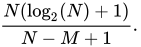
For example, when $M=201$ and $N=1024,$ Eq.3 equals $13.67,$ whereas direct evaluation of Eq.1 would require up to $201$ complex multiplications per output sample, the worst case being when both $x$ and $h$ are complex-valued. Also note that for any given $M,$ Eq.3 has a minimum with respect to $N.$ Figure 2 is a graph of the values of $N$ that minimize Eq.3 for a range of filter lengths ( $M$ ).

Instead of Eq.1, we can also consider applying Eq.2 to a long sequence of length $N_{x}$ samples. The total number of complex multiplications would be:

$N_{x}\cdot (\log _{2}(N_{x})+1).$

Comparatively, the number of complex multiplications required by the pseudocode algorithm is:

$N_{x}\cdot (\log _{2}(N)+1)\cdot {\frac {N}{N-M+1}}.$

Hence the cost of the overlap-add method scales almost as 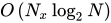$O\left(N_{x}\log _{2}N\right)$ while the cost of a single, large circular convolution is almost $O\left(N_{x}\log _{2}N_{x}\right)$ . The two methods are also compared in Figure 3, created by MATLAB simulation. The contours are lines of constant ratio of the times it takes to perform both methods. When the overlap-add method is faster, the ratio exceeds 1, and ratios as high as 3 are seen.

Fig 3: Gain of the overlap-add method compared to a single, large circular convolution. The axes show values of signal length Nx and filter length Nh.

Watch videos about Overlap-add methodExplainers and documentaries on YouTube (opens in a new tab)

Sources and credits

This article is adapted from the Wikipedia article “Overlap-add method”, written by its contributors and licensed under CC BY-SA 4.0. Fathomly has changed the layout, removed citation markers, navigation and maintenance notices, and adjusted punctuation. This adapted version is shared under the same license. For references, see the original article.

Images, from Wikimedia Commons:

Overlap-add algorithm.svg by Bob K, CC0
FFT size vs filter length for Overlap-add convolution.svg by Bob K, CC0
Gain oa method.png by Paolo Serena, University of Parma (Italy) / Paolostar at en.wikipedia, Public domain

Fathomly is not affiliated with or endorsed by the Wikimedia Foundation. Spotted a problem? Tell us.

Overlap-add method

01Algorithm

02Pseudocode

03Efficiency considerations

Sources and credits

Related topics

Overlap-save method

Circular convolution