Encyclopedia

N-vector model

Wikipedia contributorsAdapted for Fathomly · View authors

2 min read
Source updated February 6, 2026

In statistical mechanics, the n-vector model or O(n) model is a simple system of interacting spins on a crystalline lattice. It was developed by H. Eugene Stanley as a generalization of the Ising model, XY model and Heisenberg model.

01Definition

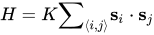
In the n-vector model, n-component unit-length classical spins $\mathbf {s} _{i}$ are placed on the vertices of a d-dimensional lattice. The Hamiltonian of the n-vector model is given by:

$H=K{\sum }_{\langle i,j\rangle }\mathbf {s} _{i}\cdot \mathbf {s} _{j}$

where the sum runs over all pairs of neighboring spins $\langle i,j\rangle$ and $\cdot$ denotes the standard Euclidean inner product. Special cases of the n-vector model are:

$n=0$ : The self-avoiding walk

$n=1$ : The Ising model

$n=2$ : The XY model

$n=3$ : The Heisenberg model

$n=4$ : Toy model for the Higgs sector of the Standard Model

The general mathematical formalism used to describe and solve the n-vector model and certain generalizations are developed in the article on the Potts model.

The Hamiltonian of the n-vector model is also the same as the potential term of the quantum rotor model.

02Reformulation as a loop model

In a small coupling expansion, the weight of a configuration may be rewritten as

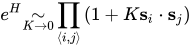
$e^{H}{\underset {K\to 0}{\sim }}\prod _{\langle i,j\rangle }\left(1+K\mathbf {s} _{i}\cdot \mathbf {s} _{j}\right)$

Integrating over the vector $\mathbf {s} _{i}$ gives rise to expressions such as

$\int d\mathbf {s} _{i}\ \prod _{j=1}^{4}\left(\mathbf {s} _{i}\cdot \mathbf {s} _{j}\right)=\left(\mathbf {s} _{1}\cdot \mathbf {s} _{2}\right)\left(\mathbf {s} _{3}\cdot \mathbf {s} _{4}\right)+\left(\mathbf {s} _{1}\cdot \mathbf {s} _{4}\right)\left(\mathbf {s} _{2}\cdot \mathbf {s} _{3}\right)+\left(\mathbf {s} _{1}\cdot \mathbf {s} _{3}\right)\left(\mathbf {s} _{2}\cdot \mathbf {s} _{4}\right)$

which is interpreted as a sum over the 3 possible ways of connecting the vertices $1,2,3,4$ pairwise using 2 lines going through vertex $i$ . Integrating over all vectors, the corresponding lines combine into closed loops, and the partition function becomes a sum over loop configurations:

$Z=\sum _{L\in {\mathcal {L}}}K^{E(L)}n^{|L|}$

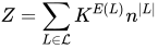
where ${\mathcal {L}}$ is the set of loop configurations, with $|L|$ the number of loops in the configuration $L$ , and $E(L)$ the total number of lattice edges.

In two dimensions, it is common to assume that loops do not cross: either by choosing the lattice to be trivalent, or by considering the model in a dilute phase where crossings are irrelevant, or by forbidding crossings by hand. The resulting model of non-intersecting loops can then be studied using powerful algebraic methods, and its spectrum is exactly known. Moreover, the model is closely related to the random cluster model, which can also be formulated in terms of non-crossing loops. Much less is known in models where loops are allowed to cross, and in higher than two dimensions.

03Continuum limit

The continuum limit can be understood to be the sigma model. This can be easily obtained by writing the Hamiltonian in terms of the product

$-{\tfrac {1}{2}}(\mathbf {s} _{i}-\mathbf {s} _{j})\cdot (\mathbf {s} _{i}-\mathbf {s} _{j})=\mathbf {s} _{i}\cdot \mathbf {s} _{j}-1$

where $\mathbf {s} _{i}\cdot \mathbf {s} _{i}=1$ is the "bulk magnetization" term. Dropping this term as an overall constant factor added to the energy, the limit is obtained by defining the Newton finite difference as

$\delta _{h}[\mathbf {s} ](i,j)={\frac {\mathbf {s} _{i}-\mathbf {s} _{j}}{h}}$

on neighboring lattice locations $i,j.$ Then $\delta _{h}[\mathbf {s} ]\to \nabla _{\mu }\mathbf {s}$ in the limit $h\to 0$ , where $\nabla _{\mu }$ is the gradient in the $(i,j)\to \mu$ direction. Thus, in the limit,

$-\mathbf {s} _{i}\cdot \mathbf {s} _{j}\to {\tfrac {1}{2}}\nabla _{\mu }\mathbf {s} \cdot \nabla _{\mu }\mathbf {s}$

which can be recognized as the kinetic energy of the field $\mathbf {s}$ in the sigma model. One still has two possibilities for the spin $\mathbf {s}$ : it is either taken from a discrete set of spins (the Potts model) or it is taken as a point on the sphere $S^{n-1}$ ; that is, $\mathbf {s}$ is a continuously-valued vector of unit length. In the later case, this is referred to as the $O(n)$ non-linear sigma model, as the rotation group $O(n)$ is group of isometries of $S^{n-1}$ , and obviously, $S^{n-1}$ isn't "flat", i.e. isn't a linear field.

04Conformal field theory

At the critical temperature and in the continuum limit, the model gives rise to a conformal field theory called the critical O(n) model. This CFT can be analyzed using expansions in the dimension d or in n, or using the conformal bootstrap approach. Its conformal data are functions of d and n, on which many results are known.

Watch videos about N-vector modelExplainers and documentaries on YouTube (opens in a new tab)

Sources and credits

This article is adapted from the Wikipedia article “N-vector model”, written by its contributors and licensed under CC BY-SA 4.0. Fathomly has changed the layout, removed citation markers, navigation and maintenance notices, and adjusted punctuation. This adapted version is shared under the same license. For references, see the original article.

Fathomly is not affiliated with or endorsed by the Wikimedia Foundation. Spotted a problem? Tell us.