Encyclopedia

Random cluster model

Type of random graph

Wikipedia contributorsAdapted for Fathomly · View authors

4 min read
Source updated June 23, 2026

In statistical mechanics, probability theory, graph theory, etc. the random cluster model is a random graph that generalizes and unifies the Ising model, Potts model, and percolation model. It is used to study random combinatorial structures, electrical networks, etc. It is also referred to as the RC model or sometimes the FK representation after its founders Cees Fortuin and Piet Kasteleyn. The random cluster model has a critical limit, described by a conformal field theory.

01Definition

Let $G=(V,E)$ be a graph, and $\omega :E\to \{0,1\}$ be a bond configuration on the graph that maps each edge to a value of either 0 or 1. We say that a bond is closed on edge $e\in E$ if $\omega (e)=0$ , and open if $\omega (e)=1$ . If we let $A(\omega )=\{e\in E:\omega (e)=1\}$ be the set of open bonds, then an open cluster or FK cluster is any connected component in $A(\omega )$ union the set of vertices. Note that an open cluster can be a single vertex (if that vertex is not incident to any open bonds).

Suppose an edge is open independently with probability $p$ and closed otherwise, then this is just the standard Bernoulli percolation process. The probability measure of a configuration $\omega$ is given as

$\mu (\omega )=\prod _{e\in E}p^{\omega (e)}(1-p)^{1-\omega (e)}.$

The RC model is a generalization of percolation, where each cluster is weighted by a factor of $q$ . Given a configuration $\omega$ , we let $C(\omega )$ be the number of open clusters, or alternatively the number of connected components formed by the open bonds. Then for any $q>0$ , the probability measure of a configuration $\omega$ is given as

$\mu (\omega )={\frac {1}{Z}}q^{C(\omega )}\prod _{e\in E}p^{\omega (e)}(1-p)^{1-\omega (e)}.$

Z is the partition function, or the sum over the unnormalized weights of all configurations,

$Z=\sum _{\omega \in \Omega }\left\{q^{C(\omega )}\prod _{e\in E(G)}p^{\omega (e)}(1-p)^{1-\omega (e)}\right\}.$

The partition function of the RC model is a specialization of the Tutte polynomial, which itself is a specialization of the multivariate Tutte polynomial.

02Special values of q

The parameter $q$ of the random cluster model can take arbitrary complex values. This includes the following special cases:

$q\to 0$ : linear resistance networks.
$q<1$ : negatively-correlated percolation.
$q=1$ : Bernoulli percolation, with $Z=1$ .
$q=2$ : the Ising model.
$q\in \mathbb {Z} ^{+}$ : $q$ -state Potts model.

03Edwards-Sokal representation

The Edwards-Sokal (ES) representation of the Potts model is named after Robert G. Edwards and Alan D. Sokal. It provides a unified representation of the Potts and random cluster models in terms of a joint distribution of spin and bond configurations.

Let $G=(V,E)$ be a graph, with the number of vertices being $n=|V|$ and the number of edges being $m=|E|$ . We denote a spin configuration as $\sigma \in \mathbb {Z} _{q}^{n}$ and a bond configuration as $\omega \in \{0,1\}^{m}$ . The joint measure of $(\sigma ,\omega )$ is given as

$\mu (\sigma ,\omega )=Z^{-1}\psi (\sigma )\phi _{p}(\omega )1_{A}(\sigma ,\omega ),$

where $\psi$ is the uniform measure, $\phi _{p}$ is the product measure with density $p=1-e^{-\beta }$ , and $Z$ is an appropriate normalizing constant. Importantly, the indicator function $1_{A}$ of the set

$A=\{(\sigma ,\omega ):\sigma _{i}=\sigma _{j}{\text{ for any edge }}(i,j){\text{ where }}\omega =1\}$

enforces the constraint that a bond can only be open on an edge if the adjacent spins are of the same state, also known as the SW rule.

The statistics of the Potts spins can be recovered from the cluster statistics (and vice versa), thanks to the following features of the ES representation:

The marginal measure $\mu (\sigma )$ of the spins is the Boltzmann measure of the q-state Potts model at inverse temperature $\beta$ .
The marginal measure $\phi _{p,q}(\omega )$ of the bonds is the random-cluster measure with parameters q and p.
The conditional measure $\mu (\sigma \,|\,\omega )$ of the spin represents a uniformly random assignment of spin states that are constant on each connected component of the bond arrangement $\omega$ .
The conditional measure $\phi _{p,q}(\omega \,|\,\sigma )$ of the bonds represents a percolation process (of ratio p) on the subgraph of $G$ formed by the edges where adjacent spins are aligned.
In the case of the Ising model, the probability that two vertices $(i,j)$ are in the same connected component of the bond arrangement $\omega$ equals the two-point correlation function of spins $\sigma _{i}{\text{ and }}\sigma _{j}$ , written $\phi _{p,q}(i\leftrightarrow j)=\langle \sigma _{i}\sigma _{j}\rangle$ .

Frustration

There are several complications of the ES representation once frustration is present in the spin model (e.g. the Ising model with both ferromagnetic and anti-ferromagnetic couplings in the same lattice). In particular, there is no longer a correspondence between the spin statistics and the cluster statistics, and the correlation length of the RC model will be greater than the correlation length of the spin model. This is the reason behind the inefficiency of the SW algorithm for simulating frustrated systems.

04Two-dimensional case

If the underlying graph $G$ is a planar graph, there is a duality between the random cluster models on $G$ and on the dual graph $G^{*}$ . At the level of the partition function, the duality reads

${\tilde {Z}}_{G}(q,v)=q^{|V|-|E|-1}v^{|E|}{\tilde {Z}}_{G^{*}}\left(q,{\frac {q}{v}}\right)\qquad {\text{with}}\qquad v={\frac {p}{1-p}}\quad {\text{and}}\quad {\tilde {Z}}_{G}(q,v)=(1-p)^{-|E|}Z_{G}(q,v)$

On a self-dual graph such as the square lattice, a phase transition can only occur at the self-dual coupling 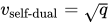$v_{\text{self-dual}}={\sqrt {q}}$ .

The random cluster model on a planar graph can be reformulated as a loop model on the corresponding medial graph. For a configuration $\omega$ of the random cluster model, the corresponding loop configuration is the set of self-avoiding loops that separate the clusters from the dual clusters. In the transfer matrix approach, the loop model is written in terms of a Temperley-Lieb algebra with the parameter $\delta =q+q^{-1}$ . In two dimensions, the random cluster model is therefore closely related to the O(n) model, which is also a loop model.

In two dimensions, the critical random cluster model is described by a conformal field theory with the central charge

$c=13-6\beta ^{2}-6\beta ^{-2}\qquad {\text{with}}\qquad q=4\cos ^{2}(\pi \beta ^{2})\ .$

Known exact results include the conformal dimensions of the fields that detect whether a point belongs to an FK cluster or a spin cluster. In terms of Kac indices, these conformal dimensions are respectively $2h_{0,{\frac {1}{2}}}$ and $2h_{{\frac {1}{2}},0}$ , corresponding to the fractal dimensions $2-2h_{0,{\frac {1}{2}}}$ and $2-2h_{{\frac {1}{2}},0}$ of the clusters.

05History and applications

RC models were introduced in 1969 by Fortuin and Kasteleyn, mainly to solve combinatorial problems. After their founders, it is sometimes referred to as FK models. In 1971 they used it to obtain the FKG inequality. Post 1987, interest in the model and applications in statistical physics reignited. It became the inspiration for the Swendsen-Wang algorithm describing the time-evolution of Potts models. Michael Aizenman and coauthors used it to study the phase boundaries in 1D Ising and Potts models.

Watch videos about Random cluster modelExplainers and documentaries on YouTube (opens in a new tab)

Sources and credits

This article is adapted from the Wikipedia article “Random cluster model”, written by its contributors and licensed under CC BY-SA 4.0. Fathomly has changed the layout, removed citation markers, navigation and maintenance notices, and adjusted punctuation. This adapted version is shared under the same license. For references, see the original article.

Fathomly is not affiliated with or endorsed by the Wikimedia Foundation. Spotted a problem? Tell us.

Random cluster model

01Definition

02Special values of q

03Edwards-Sokal representation

Frustration

04Two-dimensional case

05History and applications

Sources and credits

Related topics

Tutte polynomial

Ising model

Random graph