Encyclopedia

Modular decomposition

Recursively splitting a graph into subsets of nodes

Wikipedia contributorsAdapted for Fathomly · View authors

9 min read
Source updated October 31, 2025

In graph theory, the modular decomposition is a decomposition of a graph into subsets of vertices called modules. A module is a generalization of a connected component of a graph. Unlike connected components, however, one module can be a proper subset of another. Modules therefore lead to a recursive (hierarchical) decomposition of the graph, instead of just a partition.

There are variants of modular decomposition for undirected graphs and directed graphs. For each undirected graph, this decomposition is unique.

This notion can be generalized to other structures (for example directed graphs) and is useful to design efficient algorithms for the recognition of some graph classes, for finding transitive orientations of comparability graphs, for optimization problems on graphs, and for graph drawing.

01Modules

As the notion of modules has been rediscovered in many areas, modules have also been called autonomous sets, homogeneous sets, stable sets, clumps, committees, externally related sets, intervals, nonsimplifiable subnetworks, and partitive sets (Brandstädt, Le & Spinrad 1999). Perhaps the earliest reference to them, and the first description of modular quotients and the graph decomposition they give rise to appeared in (Gallai 1967).

A module of a graph is a generalization of a connected component. A connected component has the property that it is a set $X$ of vertices such that every member of $X$ is a non-neighbor of every vertex not in $X$ . (It is a union of connected components if and only if it has this property.) More generally, $X$ is a module if, for each vertex $v\not \in X$ , either every member of $X$ is a non-neighbor of $v$ or every member of $X$ is a neighbor of $v$ .

Equivalently, $X$ is a module if all members of $X$ have the same set of neighbors among vertices not in $X$ .

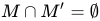
Contrary to the connected components, the modules of a graph are the same as the modules of its complement, and modules can be "nested": one module can be a proper subset of another. Note that the set $V$ of vertices of a graph is a module, as are its one-element subsets and the empty set; these are called the trivial modules. A graph may or may not have other modules. A graph is called prime if all of its modules are trivial.

Despite these differences, modules preserve a desirable property of connected components, which is that many properties of the subgraph $G[X]$ induced by a connected component $X$ are independent of the rest of the graph. A similar phenomenon also applies to the subgraphs induced by modules.

The modules of a graph are therefore of great algorithmic interest. A set of nested modules, of which the modular decomposition is an example, can be used to guide the recursive solution of many combinatorial problems on graphs, such as recognizing and transitively orienting comparability graphs, recognizing and finding permutation representations of permutation graphs, recognizing whether a graph is a cograph and finding a certificate of the answer to the question, recognizing interval graphs and finding interval representations for them, defining distance-hereditary graphs (Spinrad, 2003) and for graph drawing (Papadopoulos, 2006). They play an important role in Lovász's celebrated proof of the perfect graph theorem (Golumbic, 1980).

For recognizing distance-hereditary graphs and circle graphs, a further generalization of modular decomposition, called the split decomposition, is especially useful (Spinrad, 2003).

To avoid the possibility of ambiguity in the above definitions, we give the following formal definitions of modules. Let $G=(V,E)$ be a graph. A set $M\subseteq V$ is a module of $G$ if the vertices of $M$ cannot be distinguished by any vertex in $V\backslash M$ , i.e., $\forall u,v\in M,\forall x\in V\backslash M$ , either $x$ is adjacent to both $u$ and $v$ or $x$ is neither adjacent to $u$ nor to $v$ .

This condition can be succinctly written as $N(u)\setminus M=N(v)\setminus M$ for all $u,v\in M$ . Here, $N(u)$ denotes the set of neighbours of $u\in V$ .

For example, $\emptyset$ , $V$ and all the singletons $\{v\}$ for $v\in V$ are modules. They are called trivial modules. A graph is prime if all its modules are trivial. Connected components of a graph $G$ , or of its complement graph are also modules of $G$ .

$M$ is a strong module of a graph $G$ if it does not overlap any other module of $G$ : $\forall M'$ module of $G$ , either $M\cap M'=\emptyset$ or $M\subseteq M'$ or $M'\subseteq M$ .

A graph, its quotient where "bags" of vertices of the graph correspond to the children of the root of the modular decomposition tree, and its full modular decomposition tree: series nodes are labeled "s", parallel nodes "//" and prime nodes "p".

02Modular quotients and factors

If $X$ and $Y$ are disjoint modules, then it is easy to see that either every member of $X$ is a neighbor of every element of $Y$ , or no member of $X$ is adjacent to any member of $Y$ . Thus, the relationship between two disjoint modules is either adjacent or nonadjacent. No relationship intermediate between these two extremes can exist.

Because of this, modular partitions of $V$ where each partition class is a module are of particular interest. Suppose $P$ is a modular partition. Since the partition classes are disjoint, their adjacencies constitute a new graph, a quotient graph $G/P$ , whose vertices are the members of $P$ . That is, each vertex of $G/P$ is a module of G, and the adjacencies of these modules are the edges of $G/P$ .

In the figure below, vertex 1, vertices 2 through 4, vertex 5, vertices 6 and 7, and vertices 8 through 11 are a modular partition. In the upper right diagram, the edges between these sets depict the quotient given by this partition, while the edges internal to the sets depict the corresponding factors.

The partitions $\{V\}$ and $\{\{x\}|x\in V\}$ are the trivial modular partitions. $G/\{V\}$ is just the one-vertex graph, while $G/\{\{x\}|x\in V\}=G$ . Suppose $X$ is a nontrivial module. Then $X$ and the one-elements subsets of $V\backslash X$ are a nontrivial modular partition of $V$ . Thus, the existence of any nontrivial modules implies the existence of nontrivial modular partitions. In general, many or all members of $P$ can be nontrivial modules.

If $P$ is a nontrivial modular partition, then $G/P$ is a compact representation of all the edges that have endpoints in different partition classes of $P$ . For each partition class $X$ in $P$ , the subgraph $G[X]$ induced by $X$ is called a factor and gives a representation of all edges with both endpoints in $X$ . Therefore, the edges of $G$ can be reconstructed given only the quotient graph $G/P$ and its factors. The term prime graph comes from the fact that a prime graph has only trivial quotients and factors.

When $G[X]$ is a factor of a modular quotient $G/P$ , it is possible that $G[X]$ can be recursively decomposed into factors and quotients. Each level of the recursion gives rise to a quotient. As a base case, the graph has only one vertex. Collectively, $G$ can be reconstructed inductively by reconstructing the factors from the bottom up, inverting the steps of the decomposition by combining factors with the quotient at each level.

In the figure below, such a recursive decomposition is represented by a tree that depicts one way of recursively decomposing factors of an initial modular partition into smaller modular partitions.

A way to recursively decompose a graph into factors and quotients may not be unique. (For example, all subsets of the vertices of a complete graph are modules, which means that there are many different ways of decomposing it recursively.) Some ways may be more useful than others.

03The modular decomposition

Fortunately, there exists such a recursive decomposition of a graph that implicitly represents all ways of decomposing it; this is the modular decomposition. It is itself a way of decomposing a graph recursively into quotients, but it subsumes all others. The decomposition depicted in the figure below is this special decomposition for the given graph.

The following is a key observation in understanding the modular decomposition:

If $X$ is a module of $G$ and $Y$ is a subset of $X$ , then $Y$ is a module of $G$ , if and only if it is a module of $G[X]$ .

In (Gallai, 1967), Gallai defined the modular decomposition recursively on a graph with vertex set $V$ , as follows:

As a base case, if $G$ only has one vertex, its modular decomposition is a single tree node.
Gallai showed that if $G$ is connected and so is its complement, then the maximal modules that are proper subsets of $V$ are a partition of $V$ . They are therefore a modular partition. The quotient that they define is prime. The root of the tree is labeled a prime node, and these modules are assigned as children of $V$ . Since they are maximal, every module not represented so far is contained in a child $X$ of $V$ . For each child $X$ of $V$ , replacing $X$ with the modular decomposition tree of $G[X]$ gives a representation of all modules of $G$ , by the key observation above.
If $G$ is disconnected, its complement is connected. Every union of connected components is a module of $G$ . All other modules are subsets of a single connected component. This represents all modules, except for subsets of connected components. For each component $X$ , replacing $X$ by the modular decomposition tree of $G[X]$ gives a representation of all modules of $G$ , by the key observation above. The root of the tree is labeled a parallel node, and it is attached in place of $X$ as a child of the root. The quotient defined by the children is the complement of a complete graph.
If the complement of $G$ is disconnected, $G$ is connected. The subtrees that are children of $V$ are defined in a way that is symmetric with the case where $G$ is disconnected, since the modules of a graph are the same as the modules of its complement. The root of the tree is labeled a serial node, and the quotient defined by the children is a complete graph.

The final tree has one-element sets of vertices of $G$ as its leaves, due to the base case. A set $Y$ of vertices of $G$ is a module if and only if it is a node of the tree or a union of children of a series or parallel node. This implicitly gives all modular partitions of $V$ . It is in this sense that the modular decomposition tree "subsumes" all other ways of recursively decomposing $G$ into quotients.

04Algorithmic issues

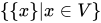
A data structure for representing the modular decomposition tree should support the operation that inputs a node and returns the set of vertices of $G$ that the node represents. An obvious way to do this is to assign to each node a list of the $k$ vertices of $G$ that it represents. Given a pointer to a node, this structure could return the set of vertices of $G$ that it represents in ${\mathcal {O}}(k)$ time. However, this data structure would require $\Theta (n^{2})$ space in the worst case.

An ${\mathcal {O}}(n)$ -space alternative that matches this performance is obtained by representing the modular decomposition tree using any standard ${\mathcal {O}}(n)$ rooted-tree data structure and labeling each leaf with the vertex of $G$ that it represents. The set represented by an internal node $v$ is given by the set of labels of its leaf descendants. It is well known that any rooted tree with $k$ leaves has at most $k-1$ internal nodes. One can use a depth-first search starting at $v$ to report the labels of leaf-descendants of $v$ in ${\mathcal {O}}(k)$ time.

Each node $X$ is a set of vertices of $G$ and, if $X$ is an internal node, the set $P$ of children of $X$ is a partition of $X$ where each partition class is a module. They therefore induce the quotient $G[X]/P$ in $G[X]$ . The vertices of this quotient are the elements of $P$ , so $G[X]/P$ can be represented by installing edges among the children of $X$ . If $Y$ and $Z$ are two members of $P$ and $u\in Y$ and $v\in Z$ , then $u$ and $v$ are adjacent in $G$ if and only if $Y$ and $Z$ are adjacent in this quotient. For any pair $\{u,v\}$ of vertices of $G$ , this is determined by the quotient at children of the least common ancestor of $\{u\}$ and $\{v\}$ in the modular decomposition tree. Therefore, the modular decomposition, labeled in this way with quotients, gives a complete representation of $G$ .

Many combinatorial problems can be solved on $G$ by solving the problem separately on each of these quotients. For example, $G$ is a comparability graph if and only if each of these quotients is a comparability graph (Gallai, 67; Möhring, 85). Therefore, to find whether a graph is a comparability graph, one need only find whether each of the quotients is. In fact, to find a transitive orientation of a comparability graph, it suffices to transitively orient each of these quotients of its modular decomposition (Gallai, 67; Möhring, 85). A similar phenomenon applies for permutation graphs, (McConnell and Spinrad '94), interval graphs (Hsu and Ma '99), perfect graphs, and other graph classes. Some important combinatorial optimization problems on graphs can be solved using a similar strategy (Möhring, 85).

Cographs are the graphs that only have parallel or series nodes in their modular decomposition tree.

The first polynomial algorithm to compute the modular decomposition tree of a graph was published in 1972 (James, Stanton & Cowan 1972) and now linear algorithms are available (McConnell & Spinrad 1999, Tedder et al. 2007, Cournier & Habib 1994).

The modular decomposition, augmented with a quotient on the children of each internal node, gives a complete representation of .

05Generalizations

Modular decomposition of directed graphs can be done in linear time (McConnell & de Montgolfier 2005).

With a small number of simple exceptions, every graph with a nontrivial modular decomposition also has a skew partition (Reed 2008).

Watch videos about Modular decompositionExplainers and documentaries on YouTube (opens in a new tab)

Sources and credits

This article is adapted from the Wikipedia article “Modular decomposition”, written by its contributors and licensed under CC BY-SA 4.0. Fathomly has changed the layout, removed citation markers, navigation and maintenance notices, and adjusted punctuation. This adapted version is shared under the same license. For references, see the original article.

Images, from Wikimedia Commons:

ModularDecomposition.png by User:Gambette, Public domain
O n ModularDecompRep.pdf by Ross m mcconnell (talk), Public domain
ModDecompQuotients.pdf by Unknown author, Public domain

Fathomly is not affiliated with or endorsed by the Wikimedia Foundation. Spotted a problem? Tell us.