Encyclopedia

Mehler kernel

Complex-valued function

Wikipedia contributorsAdapted for Fathomly · View authors

4 min read
Source updated May 20, 2026

The Mehler kernel is a complex-valued function found to be the propagator of the quantum harmonic oscillator.

It was first discovered by Mehler in 1866, and since then, as Einar Hille remarked in 1932, "has been rediscovered by almost everybody who has worked in this field".

01Mehler's formula

Mehler (1866) defined a function

$E(x,y)={\frac {1}{\sqrt {1-\rho ^{2}}}}\exp \left(-{\frac {\rho ^{2}(x^{2}+y^{2})-2\rho xy}{(1-\rho ^{2})}}\right)~,$

and showed, in modernized notation, that it can be expanded in terms of Hermite polynomials $H(\cdot )$ based on weight function $\exp(-x^{2})$ as $E(x,y)=\sum _{n=0}^{\infty }{\frac {(\rho /2)^{n}}{n!}}~{\mathit {H}}_{n}(x){\mathit {H}}_{n}(y)~.$

This result is useful, in modified form, in quantum physics, probability theory, and harmonic analysis. Equivalently, in the probabilist's Hermite polynomials: ${\frac {1}{\sqrt {1-\rho ^{2}}}}\exp \left(-{\frac {\rho ^{2}\left(x^{2}+y^{2}\right)-2\rho xy}{2\left(1-\rho ^{2}\right)}}\right)=\sum _{n=0}^{\infty }{\frac {\rho ^{n}}{n!}}~\operatorname {He} _{n}(x)\operatorname {He} _{n}(y)$ Substituting $\rho =e^{-t}$ , and letting $h_{n}:=\operatorname {He} _{n}/{\sqrt {n!}}$ , we have ${\sqrt {\tanh(t/2)}}\exp \left(-{\frac {e^{-t}(x^{2}+y^{2})-2xy}{4\sinh t}}\right)=\sum _{n=0}^{\infty }(1-e^{-t})e^{-nt}~h_{n}(x)h_{n}(y)$

02Physics version

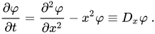
In physics, the fundamental solution, (Green's function), or propagator of the Hamiltonian for the quantum harmonic oscillator is called the Mehler kernel. It provides the fundamental solution $\varphi (x,t)$ to ${\frac {\partial \varphi }{\partial t}}={\frac {\partial ^{2}\varphi }{\partial x^{2}}}-x^{2}\varphi \equiv D_{x}\varphi ~.$

The orthonormal eigenfunctions of the operator $D$ are the Hermite functions, $\psi _{n}={\frac {H_{n}(x)\,e^{-x^{2}/2}}{\sqrt {2^{n}n!{\sqrt {\pi }}}}},$ with corresponding eigenvalues $(-2n-1)$ , furnishing particular solutions $\varphi _{n}(x,t)=e^{-(2n+1)t}~H_{n}(x)e^{-x^{2}/2}.$

The general solution is then a linear combination of these; when fitted to the initial condition $\varphi (x,0)$ , the general solution reduces to $\varphi (x,t)=\int K(x,y;t)\varphi (y,0)dy~,$ where the kernel $K$ has the separable representation $K(x,y;t)\equiv \sum _{n\geq 0}{\frac {e^{-(2n+1)t}}{{\sqrt {\pi }}2^{n}n!}}~H_{n}(x)H_{n}(y)\exp \left(-{\frac {x^{2}+y^{2}}{2}}\right)~.$

Utilizing Mehler's formula then yields ${\sum _{n\geq 0}{\frac {(\rho /2)^{n}}{n!}}H_{n}(x)H_{n}(y)\exp \left(-{\frac {x^{2}+y^{2}}{2}}\right)={\frac {1}{\sqrt {1-\rho ^{2}}}}\exp \left({\frac {4xy\rho -\left(1+\rho ^{2}\right)\left(x^{2}+y^{2}\right)}{2\left(1-\rho ^{2}\right)}}\right)}~.$

On substituting this in the expression for $K$ with the value $e^{-2t}$ for $\rho$ , Mehler's kernel finally reads

$K(x,y;t)={\frac {1}{\sqrt {2\pi \sinh(2t)}}}~\exp \left(-\coth(2t)~(x^{2}+y^{2})/2+\operatorname {csch} (2t)~xy\right).$

When $t=0$ , variables $x$ and $y$ coincide, resulting in the limiting formula necessary by the initial condition, $K(x,y;0)=\delta (x-y)~.$

As a fundamental solution, the kernel is additive, $\int dy\,K(x,y;t)K(y,z;t')=K(x,z;t{+}t')~.$

This is further related to the symplectic rotation structure of the kernel $K$ .

When using the usual physics conventions of defining the quantum harmonic oscillator instead via $i{\frac {\partial \varphi }{\partial t}}={\frac {1}{2}}\left(-{\frac {\partial ^{2}}{\partial x^{2}}}+x^{2}\right)\varphi \equiv H\varphi ,$ and assuming natural length and energy scales, then the Mehler kernel becomes the Feynman propagator $K_{H}$ which reads ${\begin{aligned}\left\langle x\right|\exp(-itH)\left|y\right\rangle &\equiv K_{H}(x,y;t)\\&={\frac {1}{\sqrt {2\pi i\sin t}}}\exp \left({\frac {i}{2\sin t}}\left(\left(x^{2}+y^{2}\right)\cos t-2xy\right)\right),\quad t<\pi ,\end{aligned}}$ i.e. $K_{H}(x,y;t)=K(x,y;it/2).$

When $t>\pi$ the $i\sin t$ in the inverse square-root should be replaced by $\left|\sin t\right|$ and $K_{H}$ should be multiplied by an extra Maslov phase factor $\exp \left(i\theta _{\text{Maslov}}\right)=\exp \left(-i{\frac {\pi }{2}}\left({\frac {1}{2}}+\left\lfloor {\frac {t}{\pi }}\right\rfloor \right)\right).$

When $t=\pi /2$ the general solution is proportional to the Fourier transform ${\mathcal {F}}$ of the initial conditions $\varphi _{0}(y)\equiv \varphi (y,0)$ since ${\begin{aligned}\varphi (x,\,t{=}{\tfrac {\pi }{2}})&=\int K_{H}(x,y;{\tfrac {\pi }{2}})\varphi (y,0)\,dy\\[1ex]&={\frac {1}{\sqrt {2\pi i}}}\int e^{-ixy}\varphi (y,0)\,dy\\[1ex]&=e^{-i\pi /4}{\mathcal {F}}[\varphi _{0}](x)~,\end{aligned}}$ and the exact Fourier transform is thus obtained from the quantum harmonic oscillator's number operator written as ${\begin{aligned}N&\equiv {\frac {1}{2}}\left(x-{\frac {\partial }{\partial x}}\right)\left(x+{\frac {\partial }{\partial x}}\right)\\&=H-{\frac {1}{2}}={\frac {1}{2}}\left(-{\frac {\partial ^{2}}{\partial x^{2}}}+x^{2}-1\right)~\end{aligned}}$ since the resulting kernel ${\begin{aligned}\left\langle x\right|\exp(-itN)\left|y\right\rangle &\equiv K_{N}(x,y;t)\\&=e^{it/2}K_{H}(x,y;t)\\&=e^{it/2}K(x,y;it/2)\end{aligned}}$ also compensates for the phase factor still arising in $K_{H}$ and $K$ , i.e. $\varphi (x,\,t{=}{\tfrac {\pi }{2}})=\int K_{N}(x,y;\pi /2)\varphi (y,0)dy={\mathcal {F}}[\varphi _{0}](x)~,$ which shows that the number operator can be interpreted via the Mehler kernel as the generator of fractional Fourier transforms for arbitrary values of $t$ , and of the conventional Fourier transform ${\mathcal {F}}$ for the particular value $t=\pi /2$ , with the Mehler kernel providing an active transform, while the corresponding passive transform is already embedded in the basis change from position to momentum space. The eigenfunctions of $N$ are the usual Hermite functions $\psi _{n}(x)$ which are therefore also Eigenfunctions of ${\mathcal {F}}$ .

03Proofs

There are many proofs of the formula.

The formula is a special case of the Hardy-Hille formula, using the fact that the Hermite polynomials are a special case of the associated Laguerre polynomials: ${\begin{aligned}H_{2n}(x)&=\left(-1\right)^{n}2^{2n}n!L_{n}^{(-1/2)}(x^{2})\\[4pt]H_{2n+1}(x)&=\left(-1\right)^{n}2^{2n+1}n!xL_{n}^{(1/2)}(x^{2})\end{aligned}}$ The formula is a special case of the Kibble-Slepian formula, so any proof of it immediately yields of proof of the Mehler formula.

Foata gave a combinatorial proof of the formula.

Hardy gave a simple proof by the Fourier integral representation of Hermite polynomials. Using the Fourier transform of the Gaussian ${\textstyle e^{-x^{2}}={\frac {1}{\sqrt {\pi }}}\int e^{-t^{2}+2ixt}dt$ , we have ${\begin{aligned}H_{n}(x)&=\left(-1\right)^{n}e^{x^{2}}{\frac {d^{n}}{dx^{n}}}e^{-x^{2}}\\&={\frac {e^{x^{2}}}{\sqrt {\pi }}}\int \left(-2it\right)^{n}e^{-t^{2}+2ixt}dt\end{aligned}}$ from which the summation $\sum _{n=0}^{\infty }{\frac {(\rho /2)^{n}}{n!}}{\mathit {H}}_{n}(x){\mathit {H}}_{n}(y)$ converts to a double integral over a summation ${\frac {e^{x^{2}+y^{2}}}{\pi }}\iint _{\mathbb {R} ^{2}}e^{-\left(t^{2}+s^{2}\right)+2i(xt+ys)}\sum _{n=0}^{\infty }{\frac {\left(-2ts\rho \right)^{n}}{n!}}dt\,ds$ which can be evaluated directly as two Gaussian integrals.

04Probability version

The result of Mehler can also be linked to probability. For this, the variables should be rescaled as $x\to x/{\sqrt {2}}$ , $y\to y/{\sqrt {2}}$ , so as to change from the "physicist's" Hermite polynomials $H(\cdot )$ (with weight function $e^{-x^{2}}$ ) to "probabilist's" Hermite polynomials $\operatorname {He} (\cdot )$ (with weight function $\exp(-x^{2}/2)$ ). They satisfy ${\begin{aligned}H_{n}(x)&=2^{\frac {n}{2}}\operatorname {He} _{n}\left({\sqrt {2}}\,x\right),&\operatorname {He} _{n}(x)&=2^{-{\frac {n}{2}}}H_{n}{\left({\frac {x}{\sqrt {2}}}\right)}.\end{aligned}}$ Then, $E$ becomes ${\frac {1}{\sqrt {1-\rho ^{2}}}}\exp \left(-{\frac {\rho ^{2}\left(x^{2}+y^{2}\right)-2\rho xy}{2\left(1-\rho ^{2}\right)}}\right)=\sum _{n=0}^{\infty }{\frac {\rho ^{n}}{n!}}~\operatorname {He} _{n}(x)\operatorname {He} _{n}(y)~.$

The left-hand side here is $p(x,y)/p(x)p(y)$ where $p(x,y)$ is the bivariate Gaussian probability density function for variables $x,y$ having zero means and unit variances: $p(x,y)={\frac {1}{2\pi {\sqrt {1-\rho ^{2}}}}}\exp \left(-{\frac {(x^{2}+y^{2})-2\rho xy}{2(1-\rho ^{2})}}\right)~,$ and $p(x),p(y)$ are the corresponding probability densities of $x$ and $y$ (both standard normal).

There follows the usually quoted form of the result (Kibble 1945) $p(x,y)=p(x)p(y)\sum _{n=0}^{\infty }{\frac {\rho ^{n}}{n!}}~\operatorname {He} _{n}(x)\operatorname {He} _{n}(y)~.$

The exponent can be written in a more symmetric form: ${\frac {1}{\sqrt {1-\rho ^{2}}}}\exp \left({\frac {\rho (x+y)^{2}}{4(1+\rho )}}-{\frac {\rho (x-y)^{2}}{4(1-\rho )}}\right)=\sum _{n=0}^{\infty }{\frac {\rho ^{n}}{n!}}~\operatorname {He} _{n}(x)\operatorname {He} _{n}(y)~.$ This expansion is most easily derived by using the two-dimensional Fourier transform of $p(x,y)$ , which is $c(iu_{1},iu_{2})=\exp \left(-{\tfrac {1}{2}}\left(u_{1}^{2}+u_{2}^{2}-2\rho u_{1}u_{2}\right)\right).$

This may be expanded as $\exp(-(u_{1}^{2}+u_{2}^{2})/2)\sum _{n=0}^{\infty }{\frac {\rho ^{n}}{n!}}(u_{1}u_{2})^{n}~.$ The Inverse Fourier transform then immediately yields the above expansion formula.

This result can be extended to the multidimensional case.

Erdélyi gave this as an integral over the complex plane $\sum _{n=0}^{\infty }{\frac {\rho ^{n}}{n!}}\operatorname {He} _{n}(x)\operatorname {He} _{n}(y)={\frac {1}{\pi t}}\iint \exp \left[-{\frac {u^{2}+v^{2}}{\rho }}+(u+iv)x+(u-iv)y-{\frac {1}{2}}(u+iv)^{2}-{\frac {1}{2}}(u-iv)^{2}\right]du\,dv.$ which can be integrated with two Gaussian integrals, yielding the Mehler formula.

05Fractional Fourier transform

Since Hermite functions $\psi _{n}$ are orthonormal eigenfunctions of the Fourier transform, ${\mathcal {F}}[\psi _{n}](y)=\left(-i\right)^{n}\psi _{n}(y)~,$ in harmonic analysis and signal processing, they diagonalize the Fourier operator, ${\mathcal {F}}[f](y)=\int dxf(x)\sum _{n\geq 0}(-i)^{n}\psi _{n}(x)\psi _{n}(y)~.$

Thus, the continuous generalization for real angle $\alpha$ can be readily defined (Wiener, 1929; Condon, 1937), the fractional Fourier transform (FrFT), with kernel ${\mathcal {F}}_{\alpha }=\sum _{n\geq 0}(-i)^{2\alpha n/\pi }\psi _{n}(x)\psi _{n}(y)~.$

This is a continuous family of linear transforms generalizing the Fourier transform, such that, for $\alpha =\pi /2$ , it reduces to the standard Fourier transform, and for $\alpha =-\pi /2$ to the inverse Fourier transform.

The Mehler formula, for $\rho =e^{-i\alpha }$ , thus directly provides ${\mathcal {F}}_{\alpha }[f](y)={\sqrt {\frac {1-i\cot(\alpha )}{2\pi }}}~e^{{\frac {i}{2}}\cot(\alpha )y^{2}/2}\int _{-\infty }^{\infty }e^{-i\left(\csc(\alpha )yx-{\frac {1}{2}}\!\cot(\alpha )x^{2}\right)}f(x)\,\mathrm {d} x\,.$ The square root is defined such that the argument of the result lies in the interval $[-\pi /2,\pi /2]$ .

If $\alpha$ is an integer multiple of $\pi$ , then the above cotangent and cosecant functions diverge. In the limit, the kernel goes to a Dirac delta function in the integrand, $\delta (x-y)$ or $\delta (x+y)$ , for $\alpha$ an even or odd multiple of $\pi$ , respectively. Since ${\mathcal {F}}^{2}[f]=f(-x)$ , ${\mathcal {F}}_{\alpha }[f]$ must be simply $f(x)$ or $f(-x)$ for $\alpha$ an even or odd multiple of $\pi$ , respectively.

Watch videos about Mehler kernelExplainers and documentaries on YouTube (opens in a new tab)

Sources and credits

This article is adapted from the Wikipedia article “Mehler kernel”, written by its contributors and licensed under CC BY-SA 4.0. Fathomly has changed the layout, removed citation markers, navigation and maintenance notices, and adjusted punctuation. This adapted version is shared under the same license. For references, see the original article.

Fathomly is not affiliated with or endorsed by the Wikimedia Foundation. Spotted a problem? Tell us.

Mehler kernel

01Mehler's formula

02Physics version

03Proofs

04Probability version

05Fractional Fourier transform

Sources and credits

Related topics

Oscillator representation

Heat kernel

Hermite polynomials