Level set
Subset of a function's domain on which its value is equal

In mathematics, a level set of a real-valued function f of n real variables is a set where the function takes on a given constant value c, that is:

When the number of independent variables is two, a level set is called a level curve, also known as contour line or isoline; so a level curve is the set of all real-valued solutions of an equation in two variables x1 and x2. When n = 3, a level set is called a level surface (or isosurface); so a level surface is the set of all real-valued roots of an equation in three variables x1, x2 and x3. For higher values of n, the level set is a level hypersurface, the set of all real-valued roots of an equation in n > 3 variables (a higher-dimensional hypersurface).
A level set is a special case of a fiber.
01Alternative names
Level sets show up in many applications, often under different names. For example, an implicit curve is a level curve, which is considered independently of its neighbor curves, emphasizing that such a curve is defined by an implicit equation. Analogously, a level surface is sometimes called an implicit surface or an isosurface.
The name isocontour is also used, which means a contour of equal height. In various application areas, isocontours have received specific names, which indicate often the nature of the values of the considered function, such as isobar, isotherm, isogon, isochrone, isoquant and indifference curve.

02Examples
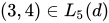
Consider the 2-dimensional Euclidean distance: 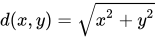




A second example is the plot of Himmelblau's function shown in the figure to the right. Each curve shown is a level curve of the function, and they are spaced logarithmically: if a curve represents 


03Level sets versus the gradient
- Theorem: If the function f is differentiable, the gradient of f at a point is either zero, or perpendicular to the level set of f at that point.
To understand what this means, imagine that two hikers are at the same location on a mountain. One of them is bold, and decides to go in the direction where the slope is steepest. The other one is more cautious and does not want to either climb or descend, choosing a path which stays at the same height. In our analogy, the above theorem says that the two hikers will depart in directions perpendicular to each other.
A consequence of this theorem (and its proof) is that if f is differentiable, a level set is a hypersurface and a manifold outside the critical points of f. At a critical point, a level set may be reduced to a point (for example at a local extremum of f ) or may have a singularity such as a self-intersection point or a cusp.

04Sublevel and superlevel sets
A set of the form

is called a sublevel set of f (or, alternatively, a lower level set or trench of f). A strict sublevel set of f is

Similarly

is called a superlevel set of f (or, alternatively, an upper level set of f). And a strict superlevel set of f is

Sublevel sets are important in minimization theory. By Weierstrass's theorem, the boundness of some non-empty sublevel set and the lower-semicontinuity of the function implies that a function attains its minimum. The convexity of all the sublevel sets characterizes quasiconvex functions.
Sources and credits
This article is adapted from the Wikipedia article “Level set”, written by its contributors and licensed under CC BY-SA 4.0. Fathomly has changed the layout, removed citation markers, navigation and maintenance notices, and adjusted punctuation. This adapted version is shared under the same license. For references, see the original article.
Images, from Wikimedia Commons:
- Level sets linear function 2d.svg by Maschen, CC0
- Trefoil knot level curves.png by Exobyte, Public domain
- Himmelblau contour.svg by Nicoguaro, CC BY 4.0
- Level grad.svg by Oleg Alexandrov, Public domain
Fathomly is not affiliated with or endorsed by the Wikimedia Foundation. Spotted a problem? Tell us.

